Demonstrate the Urban Institute quarto Theme

This is an example subtitle

Quarto at Urban

This document contains examples for how to use leverage many of Quarto’s capabilities at the Urban Institute.

1 What is Quarto?

Quarto is a tool for scientific and technical documentation. Quarto works with R, Julia, Python, and JS Observable. It can create a range of documents from simple .html documents and PDFs to full books and websites.

2 Styling Quarto

HTML documents in Quarto are styled with .scss files. PDFs are styled in Quarto with .tex files.

3 Figures and Visualizations

3.1 Figures

Quarto has powerful tools for imcluding images. It also includes native tools for adding alt text directly to images. For example, the follow code generates the subsequent image:

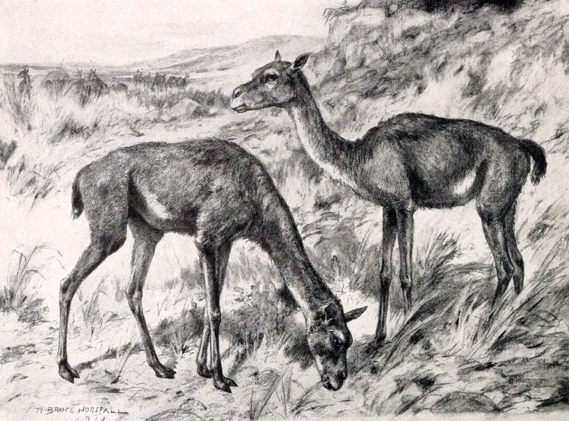![stenomylus](images/Stenomylus.jpg){#fig-stenomylus fig-alt="A sketch of two stenomylus."}

Figure 1: stenomylus

Quarto also allows for easily laying out multiple figures.

:::{#fig-camels-combo layout-ncol=2}

![stenomylus](images/Stenomylus.jpg){#fig-stenomylus}

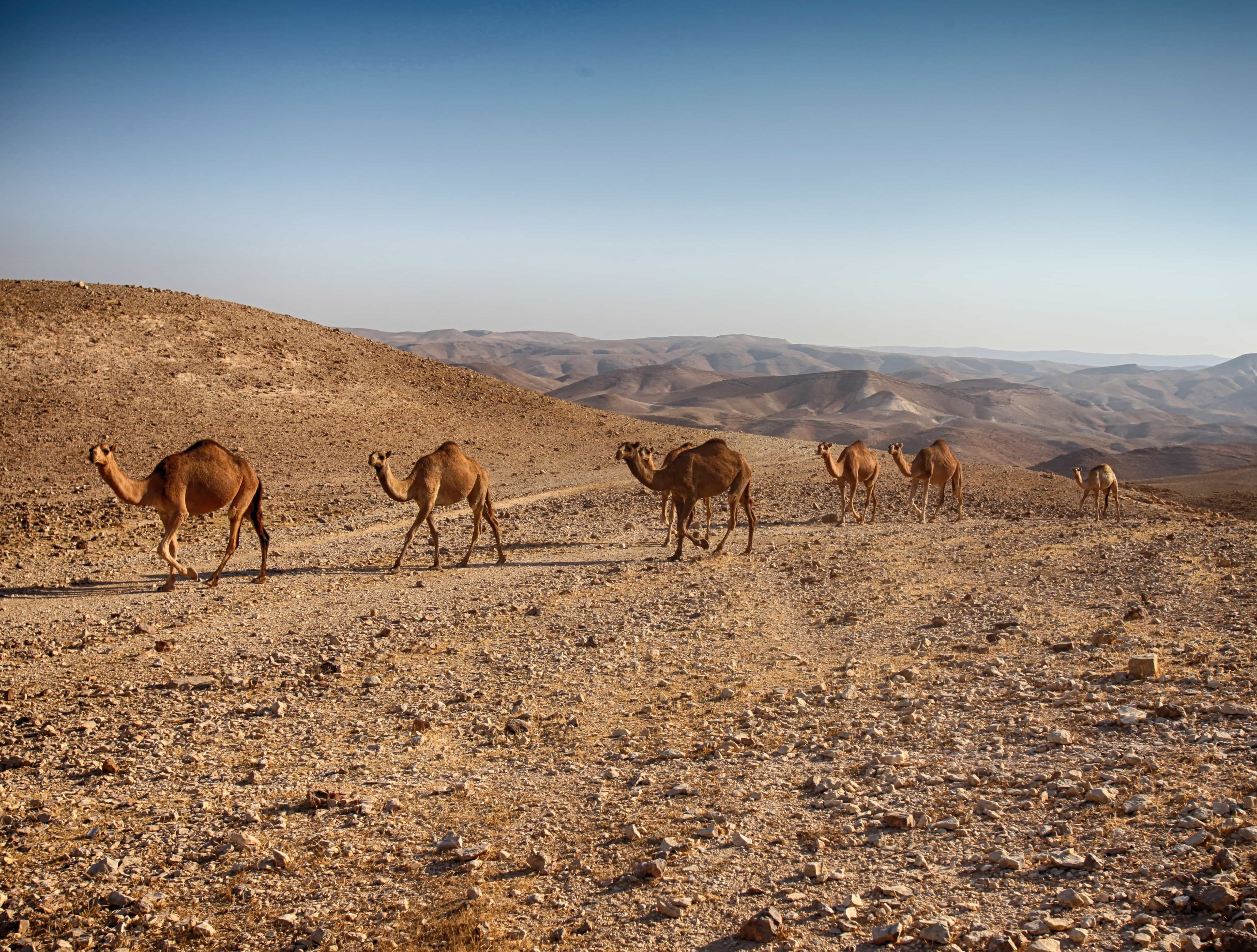![Hanno](images/camels.jpeg){#fig-camels}

Stenomylus and Camels
:::

(a) stenomylus

(b) Hanno

Figure 2: Stenomylus and Camels

3.2 Data Visualization

Quarto works well with library(urbnthemes) – the Urban Institute’s R data visualization theme.

Consider an examples using the cars dataset, which contains speed and dist for 50. Figure 3 shows two histograms displaying the distributions of speed and dist individually.

Code

ggplot(cars, aes(x = speed)) +
  geom_histogram(bins = 15) +
  labs(title = "Histogram of speeds")

ggplot(cars, aes(x = dist)) +
  geom_histogram(bins = 15) +
  labs(title = "Histogram of distances")

(a) Histogram of speeds

(b) Histogram of dists

Figure 3: Histograms of individual variables

Figure 4 displays the relationship between these two variables in a scatterplot.

Code

cars %>%
  ggplot(aes(x = speed, y = dist)) +
  geom_point(alpha = 0.3) +
  labs(title = "Cars Traveling at Higher Speeds Take Longer to Stop") +
  scatter_grid()

Figure 4: Scatterplot of speed vs. distances

3.3 Data Tables

The default for df-print is kable. This is the only type of table that works with the table references. kable works well until there is tons of data, where paged thrives.

Table 1 displays basic summary statistics for these two variables.

Code

cars %>%
  summarise(
    `Median speed` = median(speed),
    `IQR speed` = IQR(speed),
    `Median dist` = median(dist),
    `IQR dist` = IQR(dist),
    `Correlation, r` = cor(speed, dist)
  ) %>%
  kable(digits = c(0, 0, 0, 0, 2))

Table 1: Summary statistics for speed and dist (kable)

Median speed	IQR speed	Median dist	IQR dist	Correlation, r
15	7	36	30	0.81

3.4 Diagrams

Quarto has access to Mermaid and Graphviz for creating diagrams. Here is a simple example from the Quarto documentation:

flowchart LR
  A[Hard edge] --> B(Round edge)
  B --> C{Decision}
  C --> D[Result one]
  C --> E[Result two]

4 Equations

4.1 First Model

We can fit a simple linear regression model of the form shown in Equation 1.

dist = \hat{\beta}_0 + \hat{\beta}_1 \times speed + \epsilon \tag{1}

Table 2 shows the regression output for this model.

Code

dist_fit <- lm(dist ~ speed, data = cars)
  
dist_fit %>%
  tidy() %>%
  kable(digits = c(0, 0, 2, 2, 2))

Table 2: Linear regression model for predicting price from area

term	estimate	std.error	statistic	p.value
(Intercept)	-18	6.76	-2.60	0.01
speed	4	0.42	9.46	0.00

4.2 Second Model

Let’s fit a more complicated multiple linear regression model of the form shown in Equation 2.

dist = \hat{\beta}_0 + \hat{\beta}_1 \times speed + \hat{\beta}_2 \times speed ^ 2 + \epsilon \tag{2}

Table 3 shows the regression output for this model.

Code

dist_fit2 <- lm(dist ~ poly(speed, degree = 2, raw = TRUE), data = cars)
  
dist_fit2 %>%
  tidy() %>%
  kable(digits = c(0, 0, 2, 2, 2))

Table 3: Second linear regression model for predicting price from area

term	estimate	std.error	statistic	p.value
(Intercept)	2	14.82	0.17	0.87
poly(speed, degree = 2, raw = TRUE)1	1	2.03	0.45	0.66
poly(speed, degree = 2, raw = TRUE)2	0	0.07	1.52	0.14

5 Cross references

This document is littered with cross references. Cross references require labelling objects. For example:

## Cross references {#sec-cross-references}

$$
dist = \hat{\beta}_0 + \hat{\beta}_1 \times speed + \epsilon
$$ {#eq-slr}

After labeling objects, simply reference the tags with @.

The numbers in cross references automatically update when additional referenced objects are added (e.g. a table is added before table 1).

6 Footnotes

Here is an inline note¹, footnote², and a much longer footnote.³

Long notes can contain multiple paragraphs.

The notes are created with the following:

Here is an inline note^[The tooltip is pretty cool!], footnote[^1], and a much longer footnote.[^longnote]

[^1]: I suppose the footnotes are really more endnotes. 

[^longnote]: The longnote gives the ability to add very long footnotes. 
  
  Long notes can contain multiple paragraphs. 

The notes are created with the following:

7 Callouts

Note

This template is incomplete and we are always looking for help to expand it!

Warning

Caution, quarto is so powerful you may abandon LaTeX.

Important

Reproducible work is a cornerstone of quality research. Quarto makes reproducible work easy and fun.

Tip

Use library(urbntemplates) to access Urban Institute quarto templates.

Danger

Quarto may transform the way the Urban Institute communicates research.

8 Citations

Quarto simplifies adding citations to the text of a document and the reference section. It also has powerful Zotero integrations. For example, the following text generates the subsequent output.

We're going to do this analysis using literate programming [@knuth1984].

We’re going to do this analysis using literate programming (Knuth 1984).

References

Knuth, D. E. 1984. “Literate Programming.” The Computer Journal 27 (2): 97–111. https://doi.org/10.1093/comjnl/27.2.97.

Footnotes

1. The tooltip is pretty cool!

2. I suppose the footnotes are really more endnotes.

3. The longnote gives the ability to add very long footnotes.