library(nwps)
library(ggplot2)
library(urbnthemes)
library(dplyr)

set_urbn_defaults(style = "print")
#> Warning: The `size` argument of `element_line()` is deprecated as of ggplot2 3.4.0.
#> ℹ Please use the `linewidth` argument instead.
#> ℹ The deprecated feature was likely used in the urbnthemes package.
#>   Please report the issue at
#>   <https://github.com/UrbanInstitute/urbnthemes/issues>.
#> This warning is displayed once per session.
#> Call `lifecycle::last_lifecycle_warnings()` to see where this warning was
#> generated.
#> Warning: The `size` argument of `element_rect()` is deprecated as of ggplot2 3.4.0.
#> ℹ Please use the `linewidth` argument instead.
#> ℹ The deprecated feature was likely used in the urbnthemes package.
#>   Please report the issue at
#>   <https://github.com/UrbanInstitute/urbnthemes/issues>.
#> This warning is displayed once per session.
#> Call `lifecycle::last_lifecycle_warnings()` to see where this warning was
#> generated.
Introduction
The nwps package provides R functions to access the National Water Prediction Service (NWPS) API. The NWPS API offers hydrological data including:
- Gauge metadata and current status
- Stage and flow observations and forecasts
- Flood categories and impact statements
- Stage-to-flow rating curves
- National Water Model (NWM) streamflow forecasts
This vignette demonstrates how to use each of the package’s core functions.
Finding gauges
List all gauges in an area
Use nwps_gauges() to retrieve gauges within a bounding
box. The function returns an sf object with point geometries.
# Get gauges in the Washington DC area
dc_gauges <- nwps_gauges(
bbox = c(-77.5, 38.5, -76.5, 39.5),
srid = "EPSG_4326"
)
dc_gauges |>
select(lid, name, state_abbreviation, status_observed_flood_category)
#> Simple feature collection with 189 features and 4 fields
#> Geometry type: POINT
#> Dimension: XY
#> Bounding box: xmin: -77.4763 ymin: 38.54577 xmax: -76.53142 ymax: 39.48944
#> Geodetic CRS: WGS 84
#> # A tibble: 189 × 5
#> lid name state_abbreviation status_observed_floo…¹
#> <chr> <chr> <chr> <chr>
#> 1 ABPV2 Backlick Run at Armistead Bo… VA no_flooding
#> 2 ACRV2 Cameron Run at Alexandria VA out_of_service
#> 3 AFRV2 Four Mile Run at Alexandria VA no_flooding
#> 4 ALEV2 Four Mile Run above Highway … VA no_flooding
#> 5 ANAD2 Anacostia River at Washingto… DC out_of_service
#> 6 ANAV2 Accotink Creek near Annandale VA no_flooding
#> 7 APSV2 Unnamed Tributary at New Ale… VA no_flooding
#> 8 ATGV2 Unnamed Tributary above New … VA no_flooding
#> 9 AXTV2 Potomac River at Alexandria VA no_flooding
#> 10 BBSV2 Buckhall Branch at Signal Hi… VA not_defined
#> # ℹ 179 more rows
#> # ℹ abbreviated name: ¹status_observed_flood_category
#> # ℹ 1 more variable: geometry <POINT [°]>You can also filter to gauges with CatFIM (Categorical Flood Inundation Mapping) configuration:
catfim_gauges <- nwps_gauges(
  bbox = c(-77.5, 38.5, -76.5, 39.5),
  catfim = TRUE
)
#> No gauges found matching the specified criteria.

nrow(catfim_gauges)
#> [1] 0
Getting gauge details
Retrieve gauge metadata
Use nwps_gauge() to get detailed metadata for a specific
gauge by its LID or USGS ID. The function returns a list with multiple
components.
gauge <- nwps_gauge("PTTP1")

# Basic metadata (as sf object)
gauge$metadata
#> Simple feature collection with 1 feature and 12 fields
#> Geometry type: POINT
#> Dimension:     XY
#> Bounding box:  xmin: -80.01083 ymin: 40.43944 xmax: -80.01083 ymax: 40.43944
#> Geodetic CRS:  WGS 84
#> # A tibble: 1 × 13
#>   lid   usgs_id  reach_id name   description latitude longitude time_zone county
#> * <chr> <chr>    <chr>    <chr>  <chr>          <dbl>     <dbl> <chr>     <chr>
#> 1 PTTP1 03085152 3786893  Ohio … ""              40.4     -80.0 EST5EDT   Alleg…
#> # ℹ 4 more variables: in_service <lgl>, in_service_message <chr>,
#> #   forecast_reliability <chr>, geometry <POINT [°]>

# Organizational affiliations
gauge$organizations
#> # A tibble: 1 × 6
#>   rfc_abbreviation rfc_name         wfo_abbreviation wfo_name state_abbreviation
#>   <chr>            <chr>            <chr>            <chr>    <chr>
#> 1 OHRFC            Ohio River Fore… PBZ              Moon To… PA
#> # ℹ 1 more variable: state_name <chr>

# Flood category thresholds
gauge$flood_categories
#> # A tibble: 4 × 5
#>   category stage stage_units  flow flow_units
#>   <chr>    <int> <chr>       <int> <chr>
#> 1 action      18 ft          -9999 cfs
#> 2 minor       22 ft          -9999 cfs
#> 3 moderate    25 ft          -9999 cfs
#> 4 major       28 ft          -9999 cfs
View flood impact statements
Many gauges have stage-based impact statements describing what happens at different water levels:
gauge$flood_impacts
#> # A tibble: 24 × 2
#>    stage statement
#>    <dbl> <chr>
#>  1  46   Severe damage occurs in Pittsburgh with up to 15 feet of water in the …
#>  2  40   PNC Park is flooded along Federal Street.
#>  3  38   Water reaches the floor of Brunots Island Power Station.
#>  4  37   Water reaches the floor level of Rivers Casino.
#>  5  36.6 Steam distribution lines in Pittsburgh are in jeopardy. Water reaches …
#>  6  36   Serious flood damage occurs to about 500 businesses on the North Side …
#>  7  35.8 Flood waters reach the historic levels of Hurricane Agnes on June 26, …
#>  8  35   The river level reaches a critical stage for Acrisure Stadium and PNC …
#>  9  32   Mckees Rocks is affected. Flooding occurs on Neville Island.
#> 10  31   Water reaches the railroad tracks at Station Square on the South Side.…
#> # ℹ 14 more rows
Historical flood crests
You can also access historical and recent flood crest records:
gauge$flood_crests |>
  arrange(desc(stage)) |>
  head(5)
#> # A tibble: 5 × 6
#>   type     occurred_time       stage  flow preliminary old_datum
#>   <chr>    <dttm>              <dbl> <int> <chr>       <lgl>
#> 1 historic 1936-03-18 00:00:00  46       0 R           FALSE
#> 2 recent   1936-03-18 00:00:00  46       0 R           FALSE
#> 3 historic 1907-03-15 00:00:00  38.5     0 O           FALSE
#> 4 recent   1907-03-15 00:00:00  38.5     0 O           FALSE
#> 5 historic 1942-12-31 00:00:00  36.6     0 O           FALSE
Stage and flow time series
Get observed and forecast data
Use nwps_gauge_stageflow() to retrieve stage and flow
time series. By default, it returns both observed and forecast data.
stageflow <- nwps_gauge_stageflow("PTTP1")

stageflow |>
  group_by(product) |>
  summarize(
    n_obs = n(),
    min_time = min(valid_time),
    max_time = max(valid_time),
    .groups = "drop"
  )
#> # A tibble: 2 × 4
#>   product  n_obs min_time            max_time
#>   <chr>    <int> <dttm>              <dttm>
#> 1 forecast    20 2026-01-09 18:00:00 2026-01-14 12:00:00
#> 2 observed  8603 2025-12-10 18:55:00 2026-01-09 18:15:00
Visualize the hydrograph
Plot the observed and forecast stages alongside flood thresholds:
flood_cats <- gauge$flood_categories

ggplot(stageflow, aes(x = valid_time, y = primary, color = product)) +
  geom_line() +
  geom_hline(
    data = flood_cats,
    aes(yintercept = stage, linetype = category),
    color = "gray40"
  ) +
  scale_linetype_manual(
    values = c("action" = "dotted", "minor" = "dashed",
               "moderate" = "longdash", "major" = "solid")
  ) +
  labs(
    title = gauge$metadata$name,
    x = NULL,
    y = paste0("Stage (", stageflow$primary_units[1], ")"),
    color = "Product",
    linetype = "Flood Category"
  )
#> Warning: The `scale_name` argument of `discrete_scale()` is deprecated as of ggplot2
#> 3.5.0.
#> This warning is displayed once per session.
#> Call `lifecycle::last_lifecycle_warnings()` to see where this warning was
#> generated.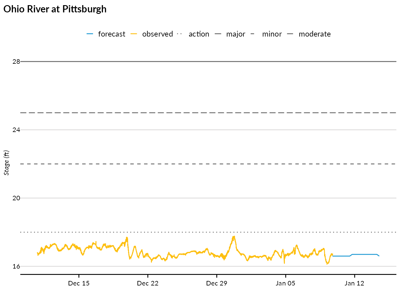
Get only observed or forecast data
You can request just one product type:
observed_only <- nwps_gauge_stageflow("PTTP1", product = "observed")
forecast_only <- nwps_gauge_stageflow("PTTP1", product = "forecast")

nrow(observed_only)
#> [1] 8604
nrow(forecast_only)
#> [1] 20
Stage-to-flow ratings
Get the rating curve
Use nwps_gauge_ratings() to retrieve the stage-to-flow
rating curve for a gauge:
ratings <- nwps_gauge_ratings("PTTP1")

head(ratings)
#> # A tibble: 6 × 4
#>   stage stage_units  flow flow_units
#>   <dbl> <chr>       <int> <chr>
#> 1  16.3 ft              0 cfs
#> 2  16.4 ft            500 cfs
#> 3  16.5 ft           2000 cfs
#> 4  16.6 ft          40009 cfs
#> 5  16.7 ft          70016 cfs
#> 6  16.8 ft          95021 cfs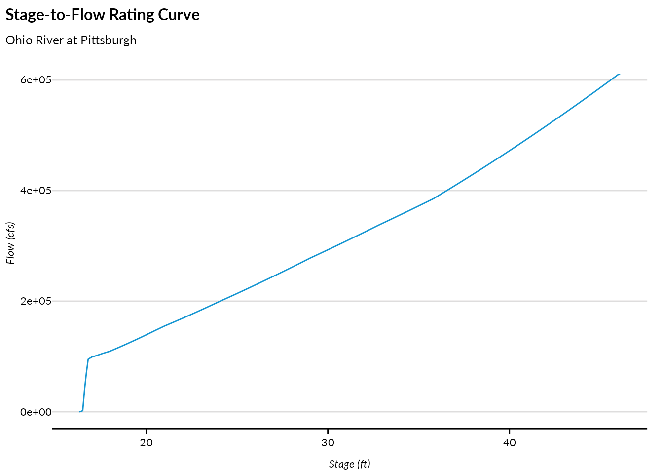
National Water Model data
The NWPS API also provides access to National Water Model (NWM) streamflow forecasts by reach.
Get reach metadata
Use nwps_reach() to retrieve metadata for an NWM
reach:
reach <- nwps_reach("22338099")

reach$metadata
#> Simple feature collection with 1 feature and 4 fields
#> Geometry type: POINT
#> Dimension:     XY
#> Bounding box:  xmin: -76.9508 ymin: 38.9149 xmax: -76.9508 ymax: 38.9149
#> Geodetic CRS:  WGS 84
#> # A tibble: 1 × 5
#>   reach_id name            latitude longitude           geometry
#> * <chr>    <chr>              <dbl>     <dbl>        <POINT [°]>
#> 1 22338099 Beaverdam Creek     38.9     -77.0 (-76.9508 38.9149)
reach$streamflow_products
#> [1] "analysis_assimilation" "short_range"           "long_range"
#> [4] "medium_range_blend"    "medium_range"
The upstream and downstream tibbles show
the reach network routing:
Get NWM streamflow forecasts
Use nwps_reach_streamflow() to retrieve streamflow
forecasts. Different forecast series are available:
-
"analysis_assimilation": Analysis and assimilation (recent past) -
"short_range": Short-range forecast (0-18 hours) -
"medium_range": Medium-range ensemble forecast (0-10 days) -
"medium_range_blend": Blended medium-range forecast -
"long_range": Long-range ensemble forecast (0-30 days)
short_range <- nwps_reach_streamflow("22338099", series = "short_range")
short_range |>
head(10)
#> # A tibble: 10 × 7
#> reach_id series member reference_time valid_time flow units
#> <chr> <chr> <chr> <dttm> <dttm> <dbl> <chr>
#> 1 22338099 short_ra… series 2026-01-09 16:00:00 2026-01-09 17:00:00 56.1 ft³/s
#> 2 22338099 short_ra… series 2026-01-09 16:00:00 2026-01-09 18:00:00 56.5 ft³/s
#> 3 22338099 short_ra… series 2026-01-09 16:00:00 2026-01-09 19:00:00 56.9 ft³/s
#> 4 22338099 short_ra… series 2026-01-09 16:00:00 2026-01-09 20:00:00 57.6 ft³/s
#> 5 22338099 short_ra… series 2026-01-09 16:00:00 2026-01-09 21:00:00 58.6 ft³/s
#> 6 22338099 short_ra… series 2026-01-09 16:00:00 2026-01-09 22:00:00 59.7 ft³/s
#> 7 22338099 short_ra… series 2026-01-09 16:00:00 2026-01-09 23:00:00 61.8 ft³/s
#> 8 22338099 short_ra… series 2026-01-09 16:00:00 2026-01-10 00:00:00 65.7 ft³/s
#> 9 22338099 short_ra… series 2026-01-09 16:00:00 2026-01-10 01:00:00 69.9 ft³/s
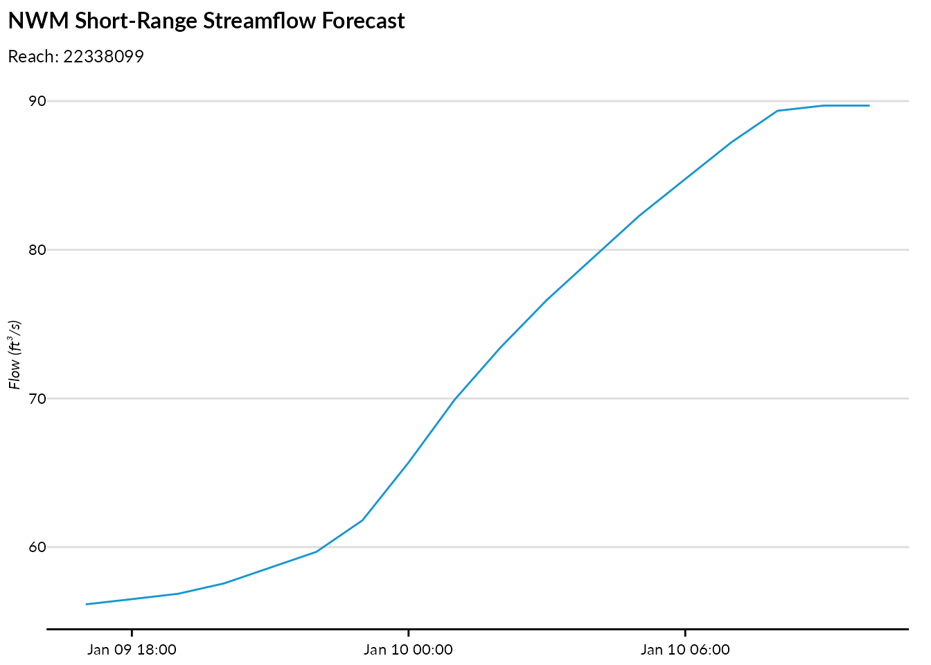
#> 10 22338099 short_ra… series 2026-01-09 16:00:00 2026-01-10 02:00:00 73.4 ft³/sVisualize NWM forecasts
ggplot(short_range, aes(x = valid_time, y = flow)) +
  geom_line() +
  labs(
    title = "NWM Short-Range Streamflow Forecast",
    subtitle = paste("Reach:", reach$metadata$reach_id),
    x = NULL,
    y = paste0("Flow (", short_range$units[1], ")")
  )
Ensemble forecasts
For medium and long-range forecasts, multiple ensemble members are available:
medium_range <- nwps_reach_streamflow("22338099", series = "medium_range")

medium_range |>
  group_by(member) |>
  summarize(n = n(), .groups = "drop")
#> # A tibble: 6 × 2
#>   member      n
#>   <chr>   <int>
#> 1 mean      204
#> 2 member1   240
#> 3 member3   204
#> 4 member4   204
#> 5 member5   204
#> 6 member6   204
SHEF product codes
Access data by PEDTS code
For more granular control, use nwps_product_stageflow()
to request data by specific SHEF PEDTS (Physical Element Data Type
Source) code:
# Get the PEDTS codes for a gauge
gauge$pedts
#> # A tibble: 1 × 2
#>   observed forecast
#>   <chr>    <chr>
#> 1 HGIR2    HGIFF

# Request observed data using PEDTS code
observed_pedts <- nwps_product_stageflow("PTTP1", "HGIRG")

head(observed_pedts)
#> # A tibble: 6 × 12
#>   pedts issued_time         wfo   time_zone valid_time
#>   <chr> <dttm>              <chr> <chr>     <dttm>
#> 1 HGIRG 2026-01-09 18:30:00 PBZ   EST5EDT   2025-12-10 18:50:00
#> 2 HGIRG 2026-01-09 18:30:00 PBZ   EST5EDT   2025-12-10 18:55:00
#> 3 HGIRG 2026-01-09 18:30:00 PBZ   EST5EDT   2025-12-10 19:00:00
#> 4 HGIRG 2026-01-09 18:30:00 PBZ   EST5EDT   2025-12-10 19:05:00
#> 5 HGIRG 2026-01-09 18:30:00 PBZ   EST5EDT   2025-12-10 19:10:00
#> 6 HGIRG 2026-01-09 18:30:00 PBZ   EST5EDT   2025-12-10 19:15:00
#> # ℹ 7 more variables: generated_time <dttm>, primary <dbl>, primary_name <chr>,
#> #   primary_units <chr>, secondary <dbl>, secondary_name <chr>,
#> #   secondary_units <chr>
System monitoring
Check API status
Use nwps_monitor() to check the system health and data
status:
status <- nwps_monitor()

# Gauges by observed flood category
status$gauge_observed
#> # A tibble: 9 × 3
#>   type     category        count
#>   <chr>    <chr>           <int>
#> 1 observed action             26
#> 2 observed low_threshold      86
#> 3 observed major               3
#> 4 observed minor               1
#> 5 observed moderate            1
#> 6 observed no_flooding      6790
#> 7 observed not_defined      3967
#> 8 observed obs_not_current   878
#> 9 observed out_of_service    804

# Gauges by forecast flood category
status$gauge_forecast
#> # A tibble: 8 × 3
#>   type     category         count
#>   <chr>    <chr>            <int>
#> 1 forecast action              42
#> 2 forecast fcst_not_current  9540
#> 3 forecast low_threshold        5
#> 4 forecast minor                1
#> 5 forecast moderate             1
#> 6 forecast no_flooding       1783
#> 7 forecast not_defined        380
#> 8 forecast out_of_service     804
The monitoring endpoint also provides information about data processing:
# HML product processing stats
status$hml_product_counts
#> # A tibble: 102 × 2
#>    time_period count
#>    <chr>       <int>
#>  1 t-10day     47087
#>  2 t-10hour     1950
#>  3 t-11day     46954
#>  4 t-11hour     1955
#>  5 t-12day     47038
#>  6 t-12hour     1951
#>  7 t-13day     47107
#>  8 t-13hour     1953
#>  9 t-14day     47099
#> 10 t-14hour     1955
#> # ℹ 92 more rows

# Long Range Outlook status
status$lro
#> # A tibble: 1 × 2
#>   current_lros current_interval
#>          <int> <chr>
#> 1         1029 JFM
Summary
The nwps package provides a complete interface to the National Water Prediction Service API:
| Function | Description |
|---|---|
nwps_gauges() |
List gauges with spatial filtering |
nwps_gauge() |
Get detailed gauge metadata |
nwps_gauge_ratings() |
Get stage-to-flow rating curves |
nwps_gauge_stageflow() |
Get observed/forecast stage and flow |
nwps_reach() |
Get NWM reach metadata |
nwps_reach_streamflow() |
Get NWM streamflow forecasts |
nwps_product_stageflow() |
Get data by SHEF PEDTS code |
nwps_monitor() |
Check system status |
For more information about the NWPS API, visit the API documentation.