egen m=mean(v1), by(v2)
bysort v2: replace m=. if _n>1
twoway bar v1 v2 
For more resources visit the STATA Users Group page on the intranet
Getting Started
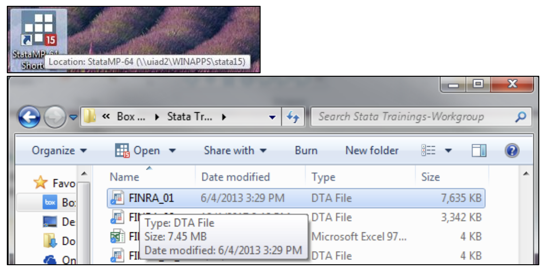
How to open Stata
It’s just like Microsoft Word in that you can open it by clicking the icon or opening a word document or template.
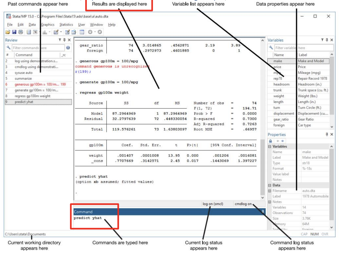
The main Stata console that opens up is your home base. Anything that you “do” will show up here. There’s a lot happening here, so for now focus on the Results window (center) and command line (bottom)
In Stata, there are three ways to set the directory (folder) that you work from:
- Access the folder via drop down menus
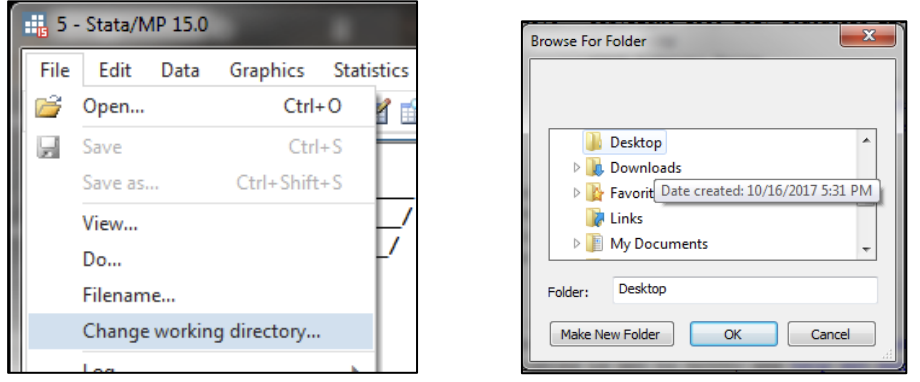
- Type the command into the command window
cd "D:\Users\clou\Desktop"- Run commands from a script (do-file)

Adding Data
The first option is that you can manually enter data or copy/paste from a spreadsheetinto browser in edit mode.
Click Data>Data Editor> Data Editor (Edit) or Type:
edit–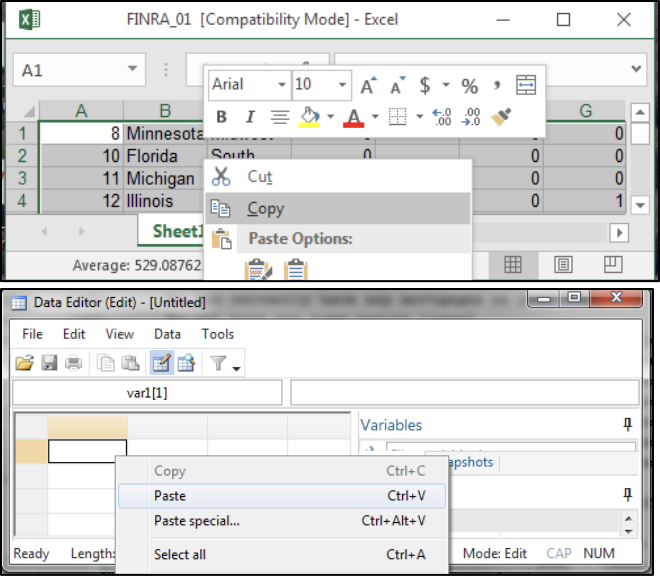
To Import from a non-stata file type (like how Microsoft word needs to convert a PDF before it can open it as a word doc) via drop-down menus go to: file>import>Excel Spreadsheet [or your file type].
The command version of this is: import excel "FINRA_01.xls", sheet("Sheet1") clear
If you just want to open an existing data set that’s already a STATA file the menu path is: file>open and the command is use "FINRA_01.dta", clear
How to look at data
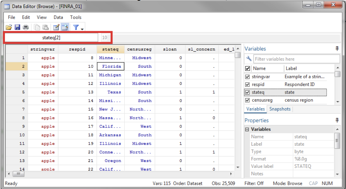
Using the data editor in browse mode (Data>Data Editor> Data Editor (Browse) or browse), you can see that data stored in STATA basically looks like a spreadsheet.
Rows = records or observations (e.g. respondents of a survey)
- Sample size (N) is the total of all the rows.
Columns = variables or characteristics (e.g. age, state)
One advantage of Stata is you can really easily search and look at groups of your variables in the \“Variables\” tab (while browsing and in the main console).
Data types
There are several different data types. This is important to know because Stata is rigid in how it stores data, and you will runinto errors/issues if your variables are not in the right type.
Numeric variables such as respid above contain discrete (integer) or continuous numeric data and appear in black (8,10,etc.). You can manipulate this data like regular numbers (i.e. add values, multiply them, etc.).
- Dummy variables: Numeric variables with the values 0 or 1 are a specific type of numeric variable called a dummy, binary, or indicator variable. A value of 1 means a record has the quality the variable’s name indicates.
String variables contain text and appear in red (apple). Always use double quotes for these values in your commands and code (“apple” above). Adding strings concatenates text and “string functions” are used to manipulate them.
Labeled numeric variables: Variables whose data appears in blue like stateq above are labeled numeric variables. They appear as text (Florida) in the browser and in the output for most commands but actually have a numeric value underlying them (10 for Florida in the above example) which must be referenced in commands/code.
- Labeled numeric variables often signify categorical or ordinal variables where the underlying numeric value does not contain useful information beyond degree (i.e. a red car is not “2x” a blue car).
Note: there are special values for missing data for numeric (. [period]) and string ( “” [empty string]) variables. The missing value for numeric data (.) is the highest numeric value and empty strings (“”) are the lowest string value in Stata, which is important for subsetting and recoding variables (more on this below). Other special values such as”don’t know,” “refused,” etc. for numeric variabls are also often coded as negative or extremely high values—refer to the data dictionary or codebook for your particular data set.
Get to know your data
One advantage of using Stata versus Excel: it’s relatively easy to run diagnostics or descriptive statistics for all or part of your data set. A crucial first step in an analysis is becoming familiar with your data. Are there missing data? Do some variables have special values? Do some records look weird? Are the variables the expected format (e.g. is age a numeric variable, not a string)? There are many issues that could arise when becoming familiar with a new data set and it’s important to refer to their documentation for help.
Describe
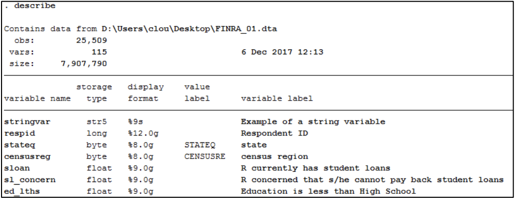
describe provides basic information about the dataset and/or its variables including name, data type, and label (usually a description) if one exists. This is an easy way to see if all the variables you want are included, and if they’re in the right format.
Codebook
codebook provides more information on variables adding in range, number missing, and number of unique values as well as example values for categorical variables and distribution for numeric variables

List
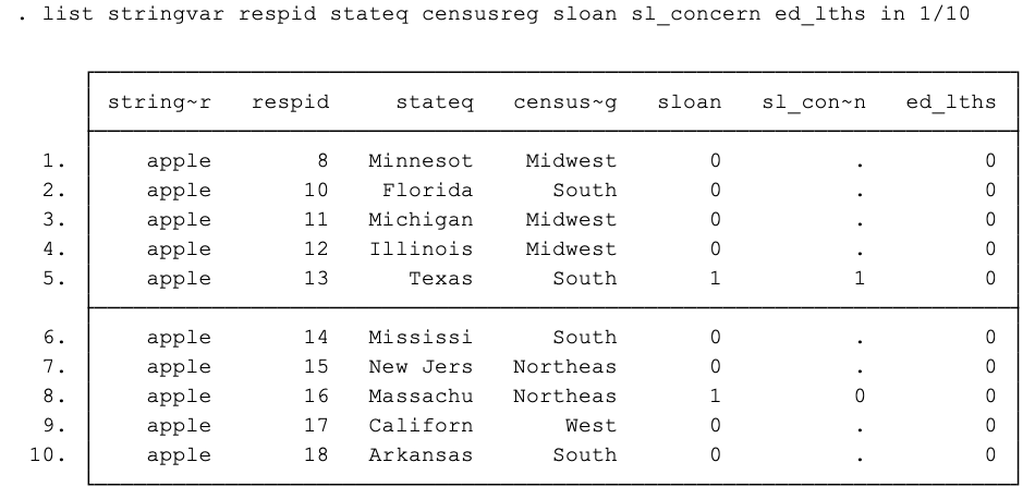
list will print a part of your data which can be useful to spot missing/special values & other issues.
Running descriptive statistics
Stata can provide summary and descriptive statistics of your data faster than in Excel. The main relationships that tell you about your data are measures of central tendency (mean, median, mode) and spread/variability (range, standard deviation, variance).
Tabluate
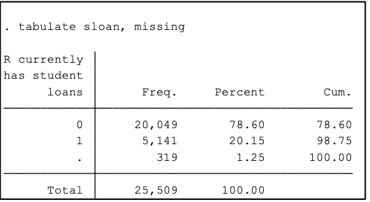
tabulate takes all a variable’s observations and gives you the frequency and percent of each value (among thetotal observations) for categorical or ordinal (e.g. gender, educational level) variables
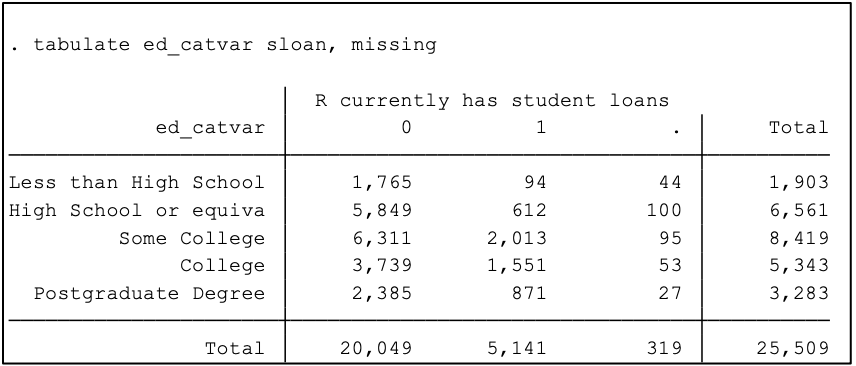
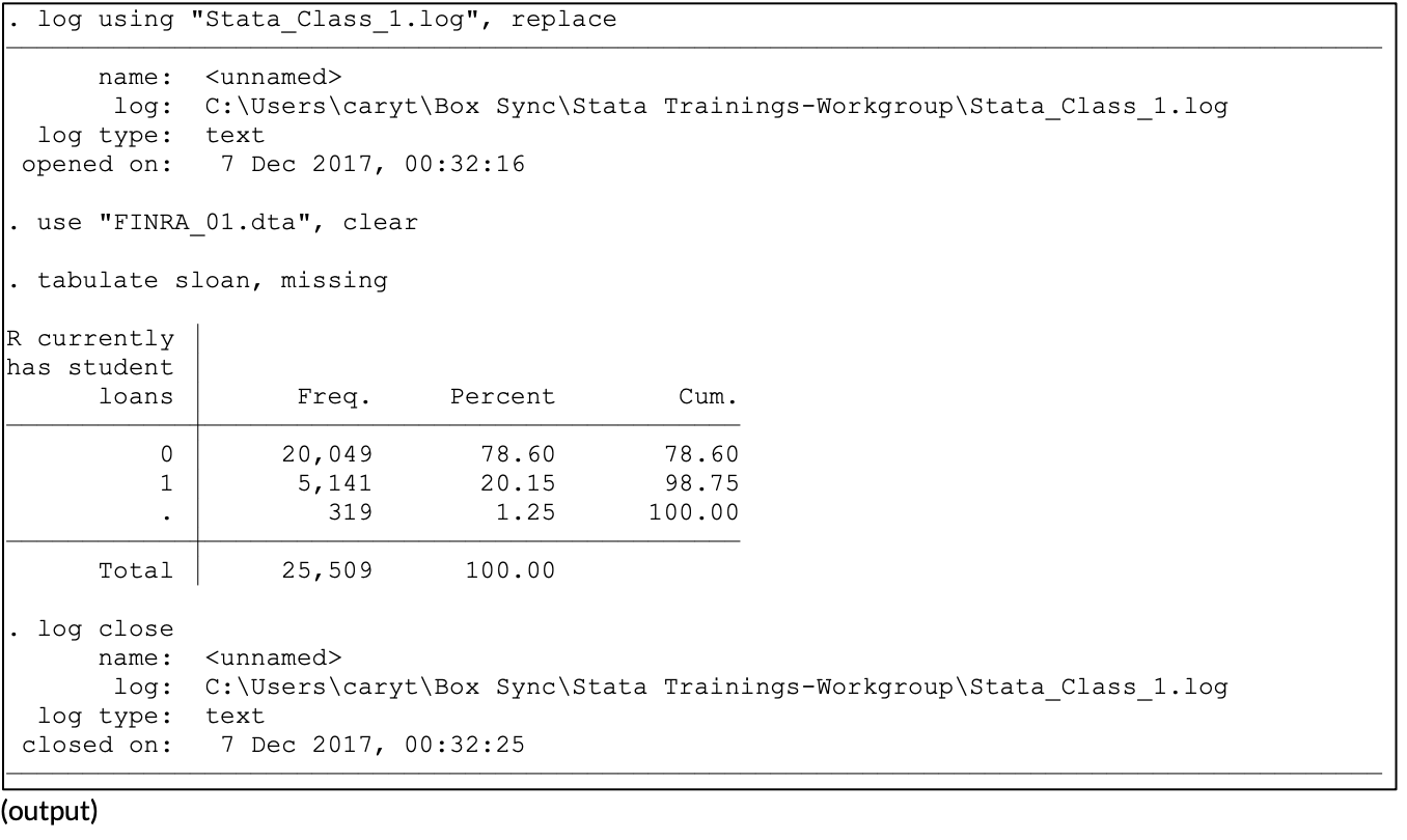
Tabulating student loans with missing option to show . values
summarize gets the number of observations, mean, standard deviation, and range and is used for discrete or continuous numeric (e.g. age, wage). The mean of a binary variable is the share of the total with that characteristic.
Summarizing the age and binary white variables

You can also crosstab two categorical/dummy variables with tabulate:
Below, we can easily see that most people who have student loans are in the categories “Some college” or “College”
Subseting
Stata can also work with a subset of your data more easily than Excel. What if I want to know the mean of everyone’s age, but only for people with postgraduate degrees? What if I want the educational attainment of only college-aged students?
Use an if conditional statement (always before the comma for options) to specify the particular observations you want a command to operate on. if expressions use common comparator operators to specify one or more conditions observations must meet for the observations to be included in the operation:
equals (==)
not equals (!= or ~=)
greater than (>)
less than (<)
greater than or equal to (>=)
less than or equal to (<=)
You can combine operators with the following Booleans:
and (&)
or (|)
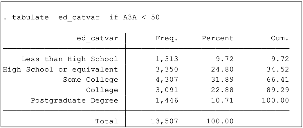
For example, we can provide statistics of education observations below age 50:
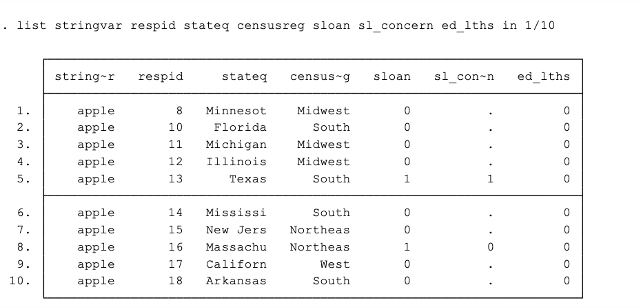
Creating an expression with in instead of if will specify a subset of observations based on their record number/order rather than a set of conditions. E.g. we already used list to print out the values of a few variables for the first ten observations by including an expression with in (in 1/10):
Adding and changing variables
So far, we’ve only looked at the variables already in the dataset. However, data rarely come perfectly. We often want to create new variables based on the variables in the dataset. It’s easy to create new variables (columns) with whatever value you would like to assign, based on the values of one or more existing variables, or more complex expressions as well as to update values. There are two main commands here:
Generate
generate: Create new variables with the generate command, a new variable name, and assign it (=) to some initial value. The command format is:
generate varname = value
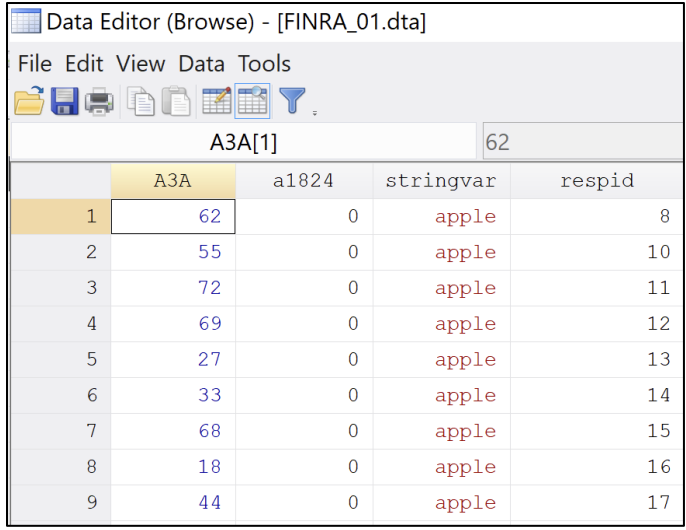
For example, if we wanted to create a new binary variable called a1824 indicating respondents ages 18-24 we would
generate a1824 = 0
Replace
replace: The replace command will update the value(s) of records for an existing variable and has similar syntax to generate:
replace varname = newvalue
It is often combined with if or in to update the values of only a subset of records:
replace a1824 = 1 if A3A >= 18 & A3A < 25
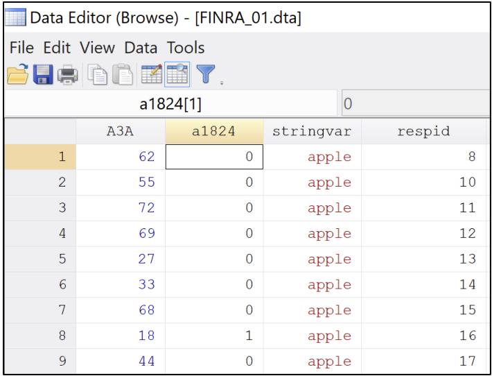
Most mistakes are human errors, and most of these are simple typos. Checking that the new variables you created have the correct range (e.g. there are no negative age values) and “look right” can save you a lot of time and trouble in the long run.
When you generate or replace variables, you can confirm whether they were created as expected by crosstabbing vs. other (original) variable(s) or summarizing.

You can also create categorical variables:

You can also create a variable whose value is a transformation of the value of another variable. For example, create age in months from age in years:

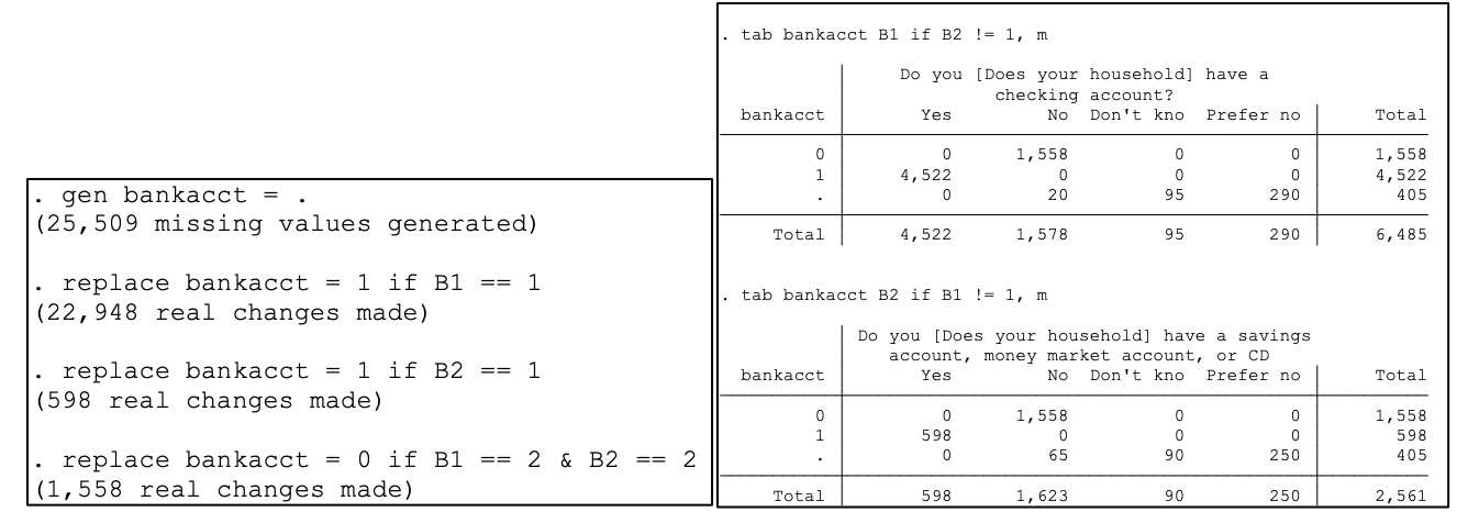
Finally, you can create cariables based on more than one other variable. Below we create a general has bank account dummy variable based on separate checking and savings account dummies. Note that it is often best practice to start by setting a new variable to missing so that missing (.), the highest value, and other special values are not accidentally coded to a valid value:
Graphics
If you are trying to make graphics, tables, or maps for publication or that are more complex than just looking at the data you have I would make a strong case for using R instead of Stata (see the R-User Group graphics guide for template code for everything data viz). There’s an urban themes package that pre-styles the graphics, and R allows for much more adaptability and customization. It’s really not hard to switch over I promise!
twoway scatter v1 v2 gives you a scatter plot of two variables, which is super useful for getting started understanding your data.
twoway lfit yvar xvar will give you a linear fit i.e. a graph of the regression line. You can overlay twoway graphs as well e.g. twoway (scatter v1 v2)(lfit v1 v2) or twoway scatter v1 v2 || lfit v1 v2
graph bar v1, over(v2) is useful for creating a bar graph of means of a continuous variable across all the categories of a categorical variable but
is much more flexible!
Any graph can be turned into a twoway graph with a bit of work and become more flexible in terms of tunable options. Even maps are twoway graphs; see here (even 3D graphs; hmap on SSC).
For all graphs, options after the comma will be helpful in labeling your graph
twoway lfit v1 v2, title(Regression line) xtitle(Treatment) ytitle(Cond. Mean Outcome)To export a graph to disk, use graph export (eps is a good format for printers; png is good for the web; see png2rtf on SSC to include a graph in a Word file). Or outfile to write out the relevant data so someone else can graph it in inferior software.
User-written commands
User-written commands are programs written by other Stata users (duh) that can be installed to act just like official Stata commands. Most of these commands are stored in Boston College’s Statistical Software Components (SSC) archive. To install them just type install ssc package .
To get a list of all of the user-written programs in the scc you can run the code:
foreach let in `c(alpha)' _ {
                ssc desc `let'
                }
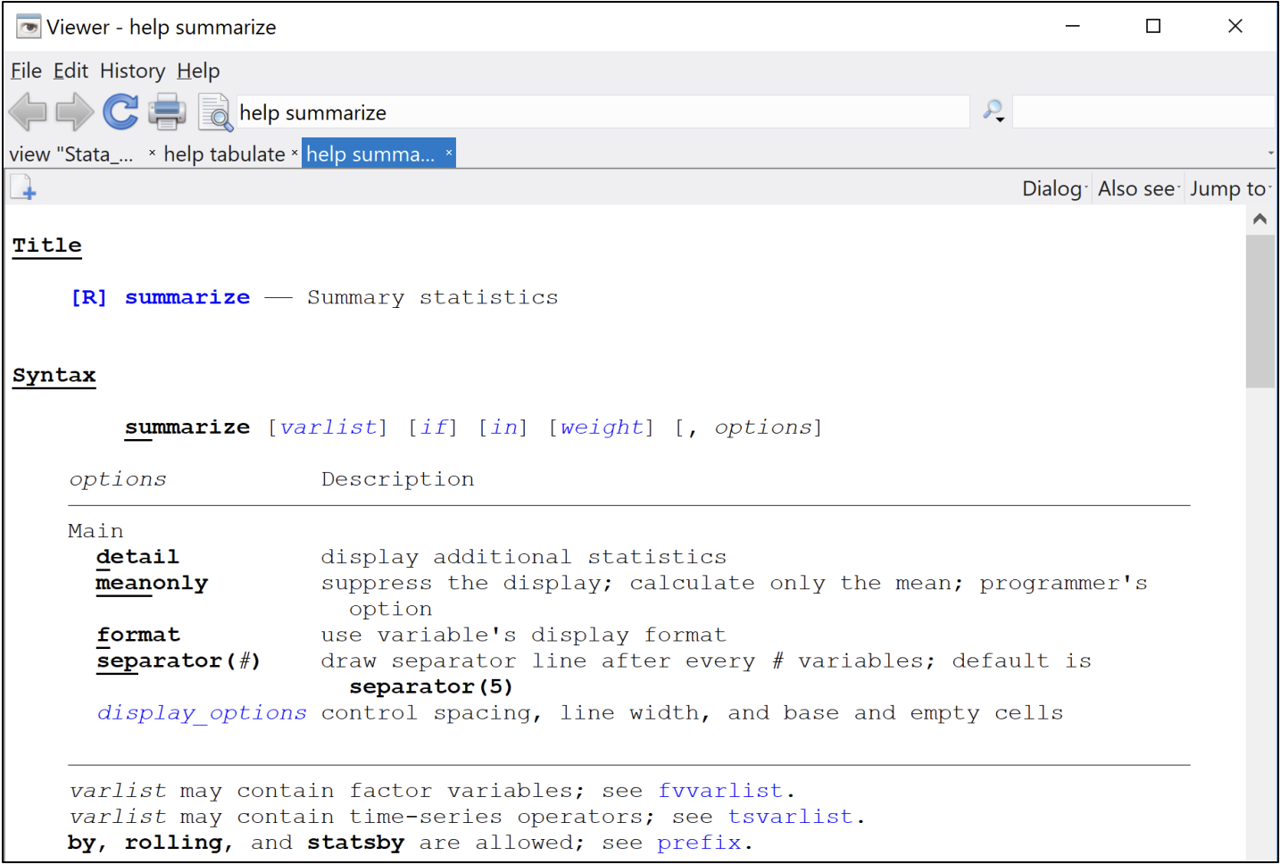
More documentation on any command is available by typing help e.g. help regress. Most help files start with a forbidding syntax diagram but have worked examples toward the bottom. If you see a command co you don’t recognize in someone else’s code, start with help co and remember the command is always the first thing on the line.
Saving work
Now that you’ve added the variables you want, you want to save your dataset so that you don’t have to recreate the variables each time you want to analyze the data. To save a Stata dataset, type:
save “Finra_02.dta”, replace
This will save whatever is in the memory (you can check browse to see). Be sure not to save it as a new name so you don’t overwrite the original data. You can also save other types of files, which we’ll get to later in a later session.
Putting it all together
Putting what you’ve just learned into a script will allow you to save, record, and replicate your work. The biggest advantage of using Stata or a similar statistical programming language— even more than statistical modeling, I think— is to allow you or others to easily save work, record results, and reproduce or modify an analysis.
Goal: set up a do file that does everything you need to do, run it, and examine the output.
When you move all the commands from the command line to Stata scripts called do files (text documents containing a series of commands) you can modify, save, and run through your entire program without typing in each line.
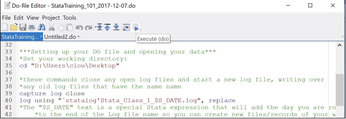
You run commands in do file by clicking the Execute (do) button that looks like a paper with a play sign (can run the whole thing or just selected lines by highlighting them) or by using the do command. You should concentrate on using do files going forward as they allow you to save and reproduce your analysis; the one above will run through this entire training and more supplementary material on top of it.
Log files
You’ve set up your do-file with all your commands (your code). You run your commands. How do you check what’s happening? How can you present it to someone without them having to open and run the program?
Start a log file at the beginning of your do file. The log file will capture whatever appears in the main results window (both the commands and their output) until you close it in a separate file under the name you specify providing a record of your work.
Generally run your entire do file through once the analysis setup is final to create a “clean” log file. It is also best practice to save a new version of your data under a different file name, often at the beginning or end of your program, so that you do not accidentally overwrite your original data source.
Help files
Help files can teach you more about basic and more advanced Stata commands and how to use them. Once you understand the syntax and setup of a help file, you can learn almost any Stata command or concept:
help summarize
Comments
Your do file code should include comments (the text in green) which will help guide you the next time you work on a project or someone new to the project or taking over your work. Specify comments with a single star (*) at the beginning of a line, double forward slash (//) to comment out the rest of a line, or /* */ for a block that will comment out everything between the stars and can go across one or more lines. Stata commands usually have to live a single line, but you can use block comments or triple-slash (///) at the end of a line to continue a command to the next line.