Chapter 10 - Tibbles
Load the libraries needed for these exercises.
library(tidyverse)10.5 - Exercises
Problem 1
How can you tell if an object is a tibble? (Hint: try printing mtcars, which is a regular data frame).
Use the is.tibble() function to determine if an object is a tibble. A tibble will also have a heading if printed to the console.
is.tibble(mtcars)## [1] FALSEis.tibble(diamonds)## [1] TRUEdiamonds## # A tibble: 53,940 x 10
## carat cut color clarity depth table price x y z
## <dbl> <ord> <ord> <ord> <dbl> <dbl> <int> <dbl> <dbl> <dbl>
## 1 0.23 Ideal E SI2 61.5 55 326 3.95 3.98 2.43
## 2 0.21 Premium E SI1 59.8 61 326 3.89 3.84 2.31
## 3 0.23 Good E VS1 56.9 65 327 4.05 4.07 2.31
## 4 0.290 Premium I VS2 62.4 58 334 4.2 4.23 2.63
## 5 0.31 Good J SI2 63.3 58 335 4.34 4.35 2.75
## 6 0.24 Very Good J VVS2 62.8 57 336 3.94 3.96 2.48
## 7 0.24 Very Good I VVS1 62.3 57 336 3.95 3.98 2.47
## 8 0.26 Very Good H SI1 61.9 55 337 4.07 4.11 2.53
## 9 0.22 Fair E VS2 65.1 61 337 3.87 3.78 2.49
## 10 0.23 Very Good H VS1 59.4 61 338 4 4.05 2.39
## # ... with 53,930 more rowsProblem 2
Compare and contrast the following operations on a data.frame and equivalent tibble. What is different? Why might the default data frame behaviours cause you frustration?
A data frame will attempt to auto-complete, while a tibble will not:
df <- data.frame(abc = 1, xyz = "a")
tib <- tibble(abc = 1, xyz = "a")

df$x
## [1] a
## Levels: atib$x## Warning: Unknown or uninitialised column: 'x'.## NULLData frames will sometimes simplify:
is.data.frame(df[, "xyz"])## [1] FALSEis.tibble(tib[, "xyz"])## [1] TRUETibble will display useful information on the data:
df[, c("abc", "xyz")]## abc xyz
## 1 1 atib[, c("abc", "xyz")]## # A tibble: 1 x 2
## abc xyz
## <dbl> <chr>
## 1 1 aProblem 3
If you have the name of a variable stored in an object, e.g. var <- "mpg", how can you extract the reference variable from a tibble?
Use [] to extract the variable and [[]] to extract the vector:
var <- 'mpg'
as.tibble(mtcars)[var]
## # A tibble: 32 x 1
## mpg
## <dbl>
## 1 21
## 2 21
## 3 22.8
## 4 21.4
## 5 18.7
## 6 18.1
## 7 14.3
## 8 24.4
## 9 22.8
## 10 19.2
## # ... with 22 more rowsas.tibble(mtcars)[[var]]## [1] 21.0 21.0 22.8 21.4 18.7 18.1 14.3 24.4 22.8 19.2 17.8 16.4 17.3 15.2
## [15] 10.4 10.4 14.7 32.4 30.4 33.9 21.5 15.5 15.2 13.3 19.2 27.3 26.0 30.4
## [29] 15.8 19.7 15.0 21.4Problem 4
Practice referring to non-syntactic names in the following data frame by:
- Extracting the variable called 1.
annoying <- tibble(
  `1` = 1:10,
  `2` = `1` * 2 + rnorm(length(`1`))
)

annoying %>%
  select(`1`)
## # A tibble: 10 x 1
## `1`
## <int>
## 1 1
## 2 2
## 3 3
## 4 4
## 5 5
## 6 6
## 7 7
## 8 8
## 9 9
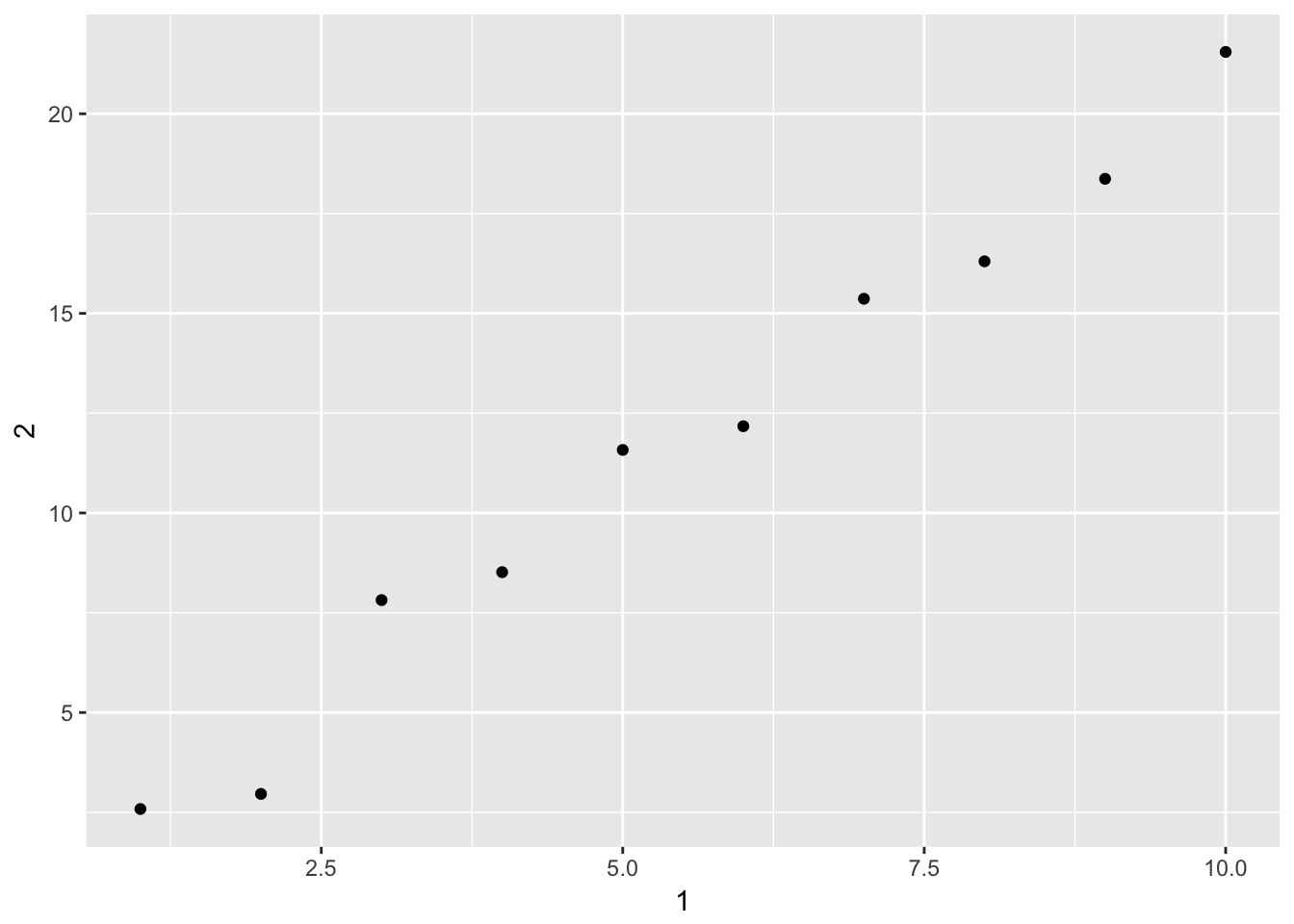
## 10 10- Plotting a scatterplot of 1 vs 2.
ggplot(annoying, aes(`1`, `2`)) +
  geom_point()
- Creating a new column called 3 which is 2 divided by 1.
annoying <- annoying %>%
mutate(`3` = `2` / `1`)- Renaming the columns to one, two and three.
annoying %>%
  select(one = `1`,
         two = `2`,
         three = `3`)
## # A tibble: 10 x 3
## one two three
## <int> <dbl> <dbl>
## 1 1 2.58 2.58
## 2 2 2.96 1.48
## 3 3 7.82 2.61
## 4 4 8.52 2.13
## 5 5 11.6 2.32
## 6 6 12.2 2.03
## 7 7 15.4 2.20
## 8 8 16.3 2.04
## 9 9 18.4 2.04
## 10 10 21.5 2.15Problem 5
What does tibble::enframe() do? When might you use it?
enframe() can be used to convert a vector or list to a tibble:
enframe(c(a = 5, b = 10))## # A tibble: 2 x 2
## name value
## <chr> <dbl>
## 1 a 5
## 2 b 10Problem 6
What option controls how many additional column names are printed at the footer of a tibble?
The tibble.max_extra_cols option controls this behavior, with a default of 100.