Chapter 7 - Exploratory Data Analysis

Load the libraries needed for these exercises.

library(tidyverse)

7.3 - Variation

Problem 1

Explore the distribution of each of the x, y, and z variables in diamonds. What do you learn? Think about a diamond and how you might decide which dimension is the length, width, and depth.

The distribution of x, y, and z generally seems to fall between 0 and 10mm, although the distributions of y and z both have much longer tails.

ggplot(data = diamonds) + 
  geom_histogram(mapping = aes(x = x), binwidth = 0.5)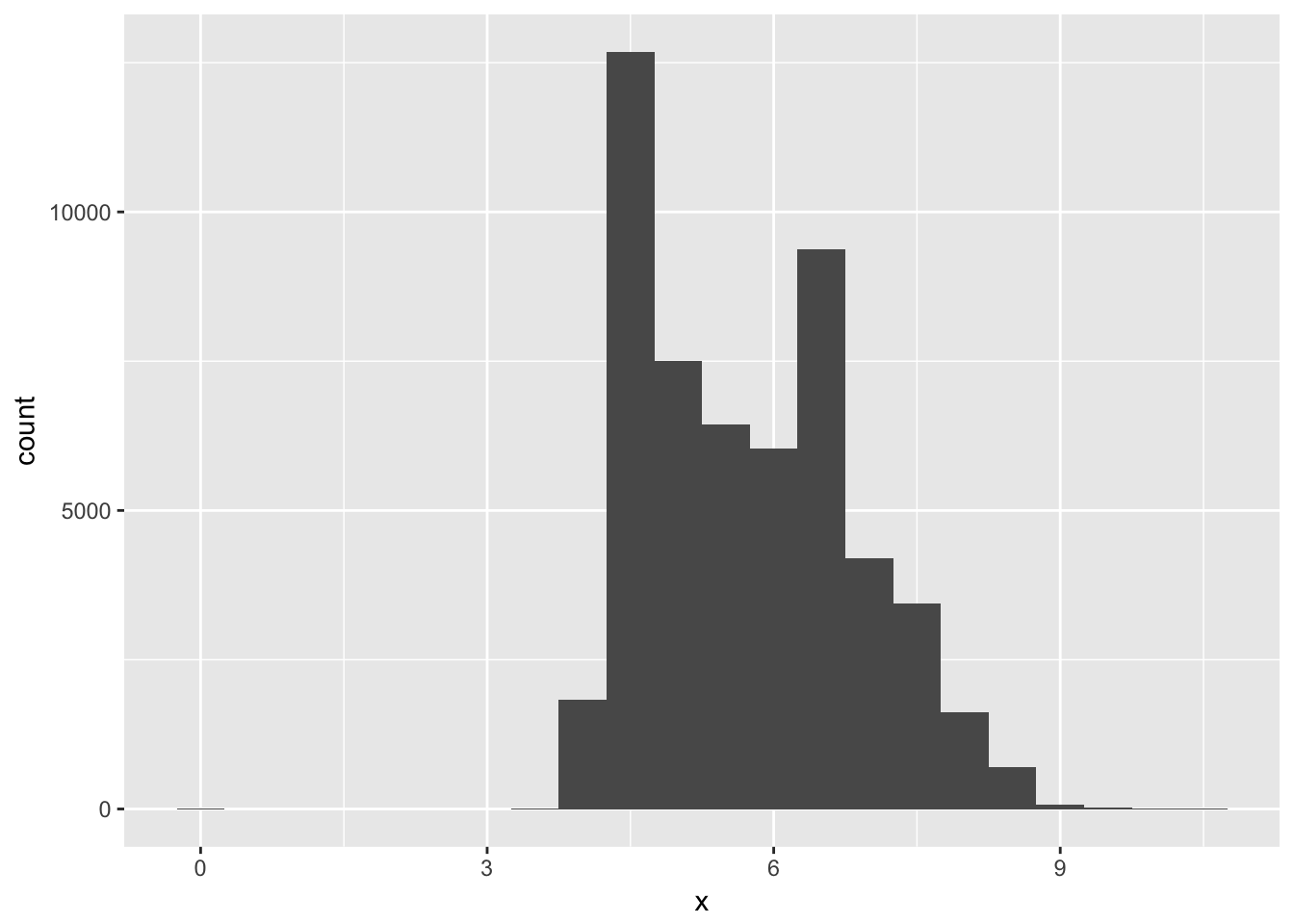

ggplot(data = diamonds) + 
  geom_histogram(mapping = aes(x = y), binwidth = 0.5)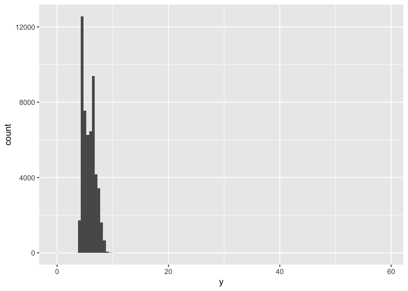

ggplot(data = diamonds) + 
  geom_histogram(mapping = aes(x = z), binwidth = 0.5)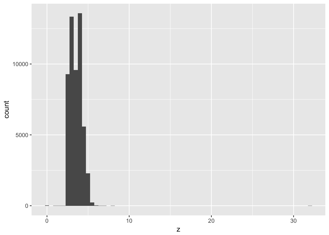

Problem 2

Explore the distribution of price. Do you discover anything unusual or surprising? (Hint: Carefully think about the binwidth and make sure you try a wide range of values.)

The price of diamonds appears to peak around $2000, followed by a long tail for the much more expensive diamonds. Narrowing the value of binwidth shows that some values are not very populated.

ggplot(data = diamonds) + 
  geom_histogram(mapping = aes(x = price), binwidth = 1000)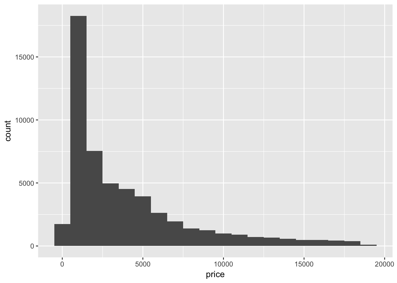

ggplot(data = diamonds) + 
  geom_histogram(mapping = aes(x = price), binwidth = 500)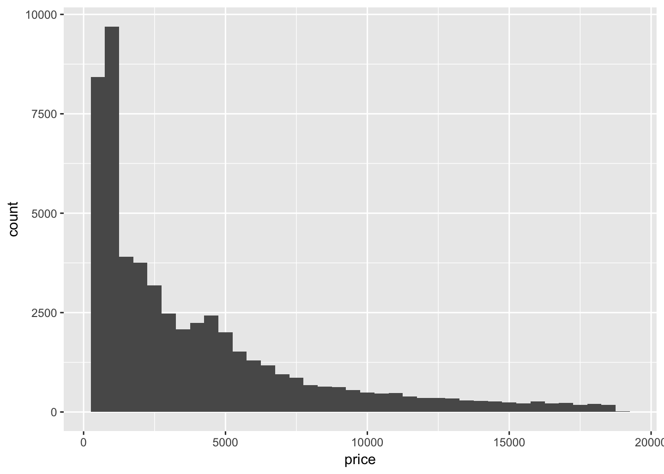

ggplot(data = diamonds) + 
  geom_histogram(mapping = aes(x = price), binwidth = 100)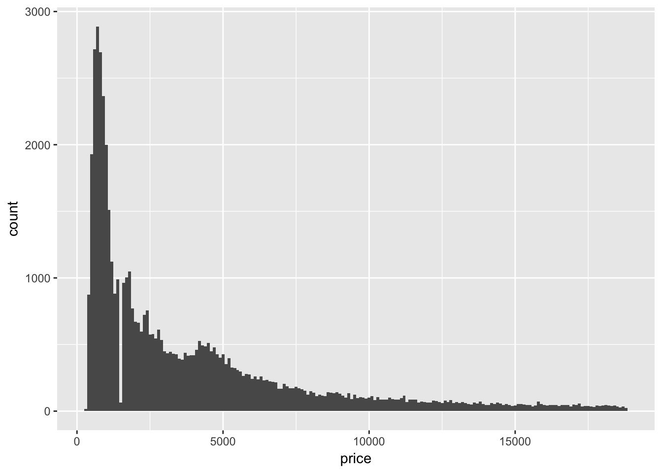

Problem 3

How many diamonds are 0.99 carat? How many are 1 carat? What do you think is the cause of the difference?

People may prefer to buy a diamond that is a full carat rather than almost a carat large. There appears to be significant rounding in the data set:

diamonds %>%
  filter(between(carat, 0.99, 1.00)) %>%
  group_by(carat) %>%
  count()

## # A tibble: 2 x 2
## # Groups:   carat [2]
##   carat     n
##   <dbl> <int>
## 1  0.99    23
## 2  1     1558

Problem 4

Compare and contrast coord_cartesian() vs xlim() or ylim() when zooming in on a histogram. What happens if you leave binwidth unset? What happens if you try and zoom so only half a bar shows?

Compare and contrast the following three graphs: while coord_cartesian() will preserve data, ylim() will drop rows that fall outside of the limits.

ggplot(diamonds) + 
  geom_histogram(mapping = aes(x = y), binwidth = 0.5)

ggplot(diamonds) + 
  geom_histogram(mapping = aes(x = y), binwidth = 0.5) +
  coord_cartesian(ylim = c(0,60))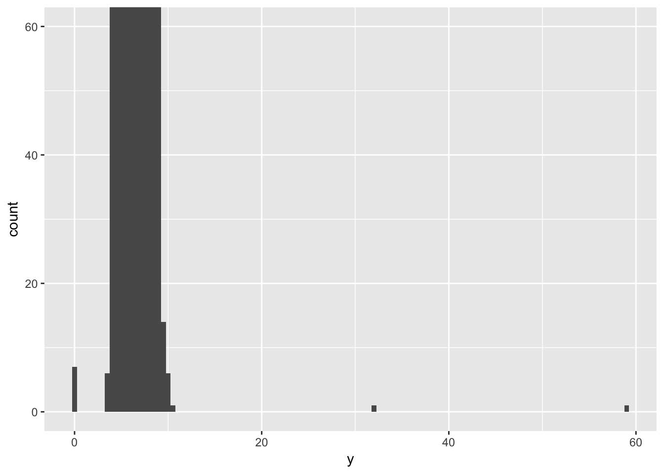

ggplot(diamonds) + 
  geom_histogram(mapping = aes(x = y), binwidth = 0.5) +
  ylim(0,60)

## Warning: Removed 11 rows containing missing values (geom_bar).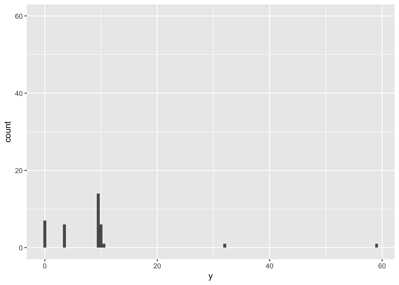

7.4 - Missing Values

Problem 1

What happens to missing values in a histogram? What happens to missing values in a bar chart? Why is there a difference?

Missing values are plotted in a bar chart but not a histogram. Remember that histograms are generally used to display numeric data, while bar charts are used for categorical data. Missing values can be considered another category to plot in a bar chart, but there is not necessarily an intuitive way to place missing values in a histogram.

diamonds %>% 
  mutate(cut = ifelse(cut == 'Fair', NA, cut)) %>%
  ggplot(aes(x=cut)) +
  geom_histogram()

## `stat_bin()` using `bins = 30`. Pick better value with `binwidth`.

## Warning: Removed 1610 rows containing non-finite values (stat_bin).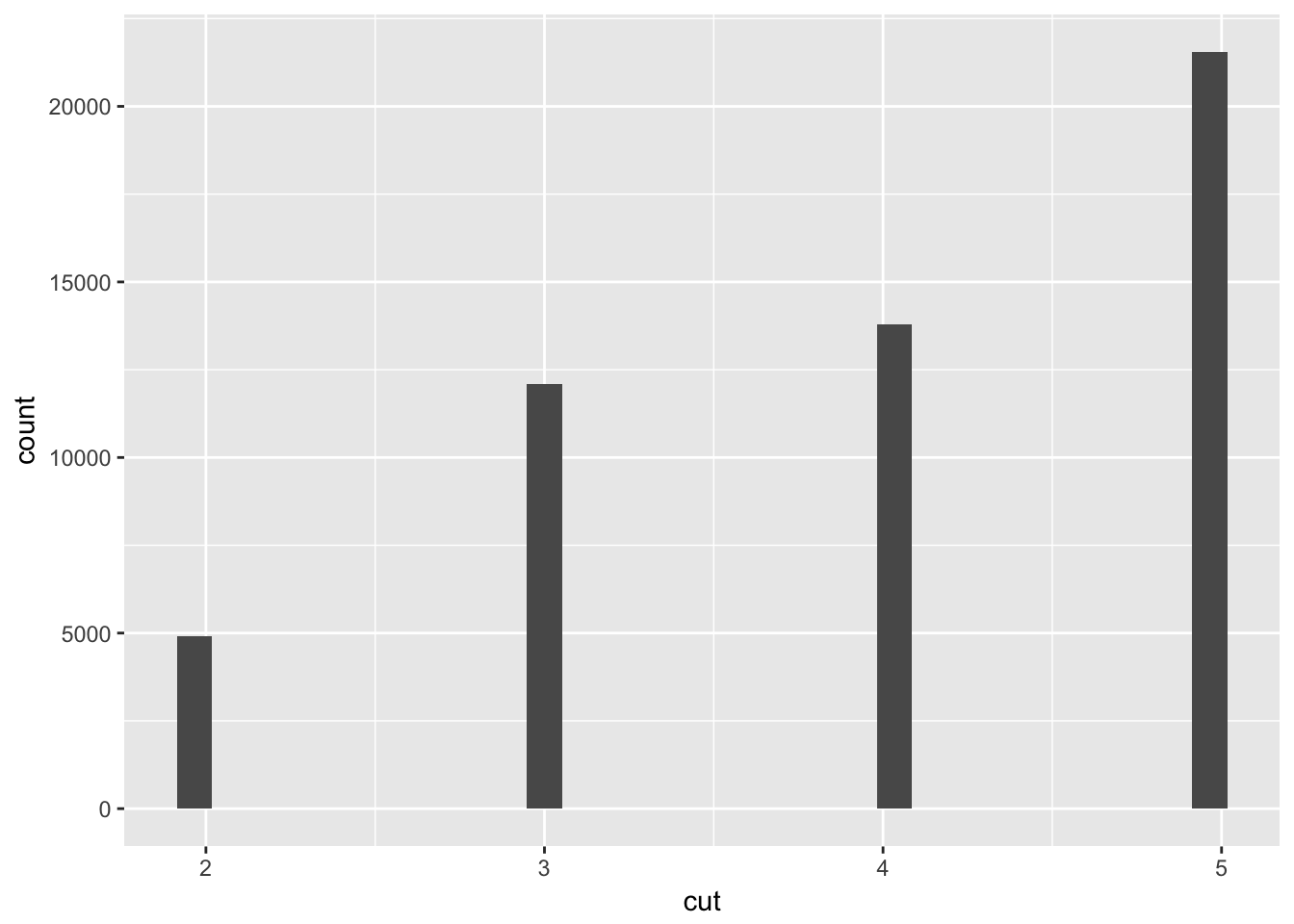

diamonds %>% 
  mutate(cut = as.character(cut)) %>%
  mutate(cut = ifelse(cut == 'Fair', NA, cut)) %>%
  ggplot(aes(x=cut)) +
  geom_bar()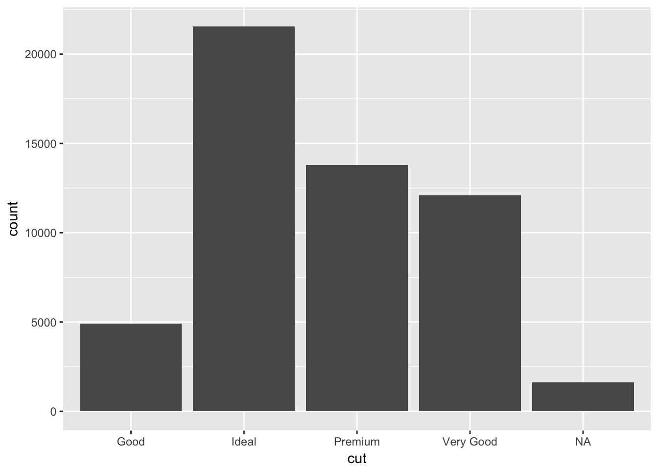

Problem 2

What does na.rm = TRUE do in mean() and sum()?

Setting na.rm = TRUE will remove missing values before executing the function.

x <- c(1, 2, 3, NA)
mean(x)

## [1] NA

mean(x, na.rm = TRUE)

## [1] 2