Economic Recovery Post Disaster

Overview

Because post-event data for the affected area will not be available for months or years, this approach identifies historical comparison—counties that experienced similar disasters and had similar pre-disaster characteristics—in the past—to highlight various recovery trajectories.

Contents:

1. The affected county’s pre-disaster economic baseline
2. Employment, business, and local government finance trajectories using an event-study framework
3. Typical PA/IHP/SBA flows from federal programs (post-disaster period only)

Notes

Critical to this approach is an observable pre-period, especially for the disaster-impacted county (which has no post-period data). But because of data lags, the pre-period will never run up through 2026 (current year at time of writing)–at best, it will go through ~2024 (ACS) or in most cases only 2023 (County Business Patterns, government finances).

Accordingly, we want our pre-period to be long–say, 8 years preceding the disaster, if possible–so that we have multiple years of observation, even for the disaster-affected county. But for our comparison counties, we are hemmed in on the other side–we want to have post-period observations for these, so the comparison disaster ideally occurs between 2018-2020, giving us 3-5 post-period years. However, this requires a pre-period dating back to as early as 2010… which is not covered in many datasets (e.g., ACS). Thus, we have a tension in identifying overlapping pre-period timelines for our comparison and affected counties due to historical data coverage.

Setup

library(climateapi)
library(tidyverse)
library(urbnthemes)
library(crosswalk)

set_urbn_defaults(style = "print")

Parameters

Define the affected county and disaster characteristics. These would be updated for each new event.

# Affected county
affected_county_fips <- "12087"
affected_county_name <- "Monroe County, FL"
affected_state <- "FL"

# Disaster characteristics
disaster_type <- "Hurricane"
disaster_year <- 2026

# Event-study window
years_before <- 6
years_after <- 4

Preceding Disasters

disasters = get_fema_disaster_declarations(api = FALSE)
disasters_affected = disasters %>%
  filter(GEOID %in% affected_county_fips, incidents_natural_hazard > 0)

---

Section 1: The Affected County Baseline Profile

Establish the pre-disaster economic conditions of the affected county.

Sociodemographic Characteristics

acs_df_2023 = arrow::read_parquet(file.path(get_box_path(), "sociodemographics", "acs", "acs_county_2023.parquet"))

acs_matching_variables = c(
  "median_household_income_universe_allraces",
  "race_personofcolor_percent",
  "population_density_land_sq_kilometer",
  "total_population_universe",
  "educational_attainment_degree_bachelors_percent")

Hazard Damages over Time

sheldus_df = get_sheldus() %>%
   summarize(.by = c(GEOID, year), damage_property_millions = sum(damage_property, na.rm = TRUE) / 1000000)

sheldus_df %>% 
  filter(GEOID %in% affected_county_fips) %>%
  ggplot(aes(x = year, y = damage_property_millions)) +
    geom_line() +
    geom_point() +
    scale_y_continuous(labels = scales::dollar_format(suffix = "M")) +
    labs(x = "Year", y = "Property damage (millions)")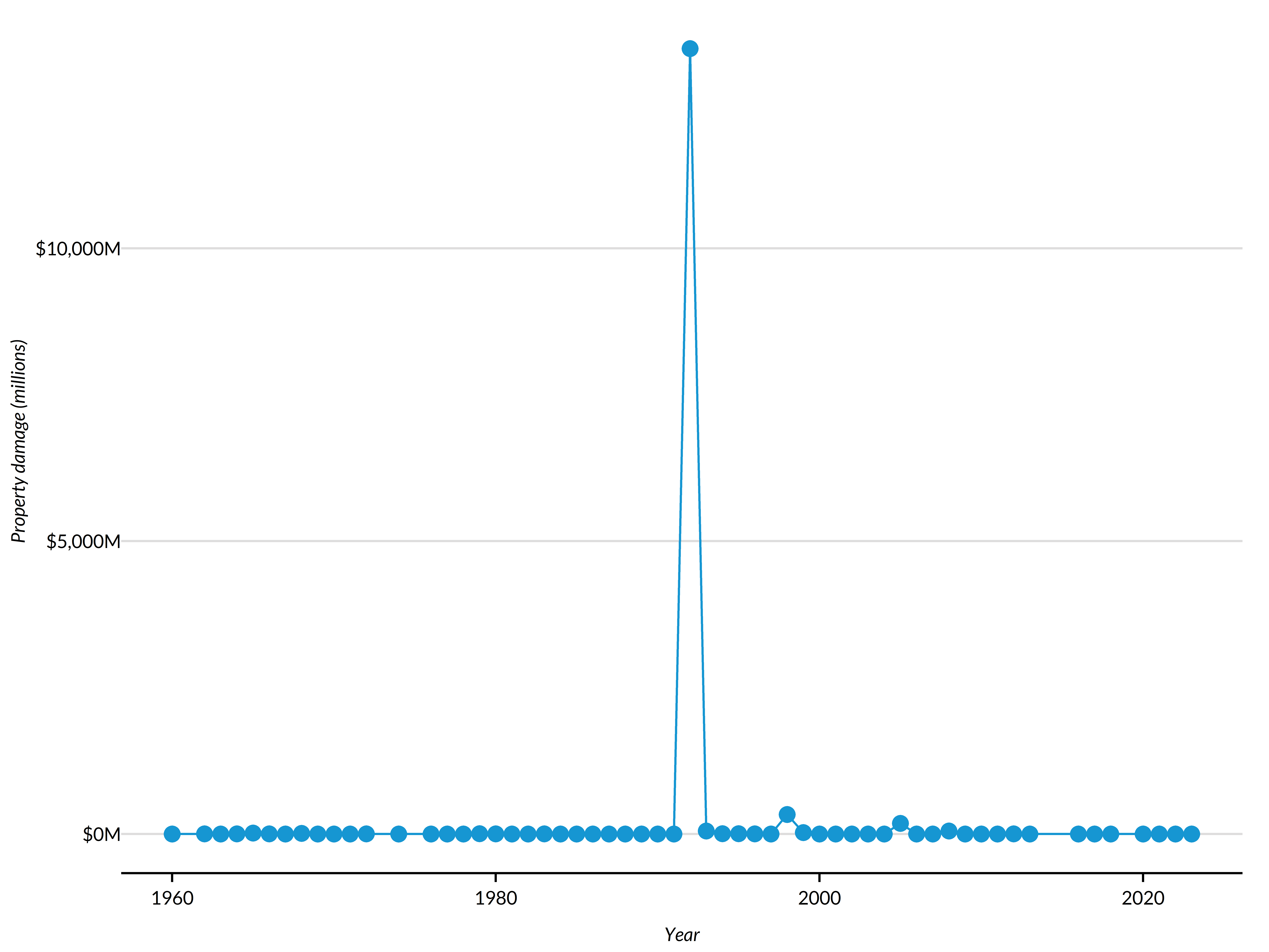

plot of chunk unnamed-chunk-4

Industry Composition over Time

Identify sectors that may be particularly vulnerable to this disaster type.

cbp_df = cache_it(
  cbp_df, 
  file_name = "cbp_2016_2023", 
  path = file.path(get_box_path(), "employment"), read = TRUE)

cbp_affected = cbp_df %>%
  mutate(
    county_fips = str_c(state, county),
    industry_label = industry %>% str_replace_all("_", " ") %>% str_to_sentence()) %>%
  filter(county_fips %in% affected_county_fips)

top_8_industries = cbp_affected %>%
  filter(year == 2023, industry != "total") %>%
  arrange(desc(employees)) %>%
  slice(1:8) %>%
  pull(industry)

cbp_prior_disaster_years = disasters_affected %>%
  filter(year_declared %in% (cbp_df$year %>% unique())) %>%
  distinct(year_declared)

cbp_affected %>%
  filter(employees > 0, industry %in% top_8_industries) %>%
  arrange(desc(employees)) %>%
  ggplot(aes(x = year, y = employees, color = industry_label, group = industry_label)) +
  geom_line() +
  geom_vline(data = cbp_prior_disaster_years, color = "grey", linetype = "dashed", aes(xintercept = year_declared)) +
  scale_y_continuous(labels = scales::comma) +
  scale_x_continuous(n.breaks = length((cbp_df$year %>% unique()))) +
  labs(y = "Employees (n)", x = "")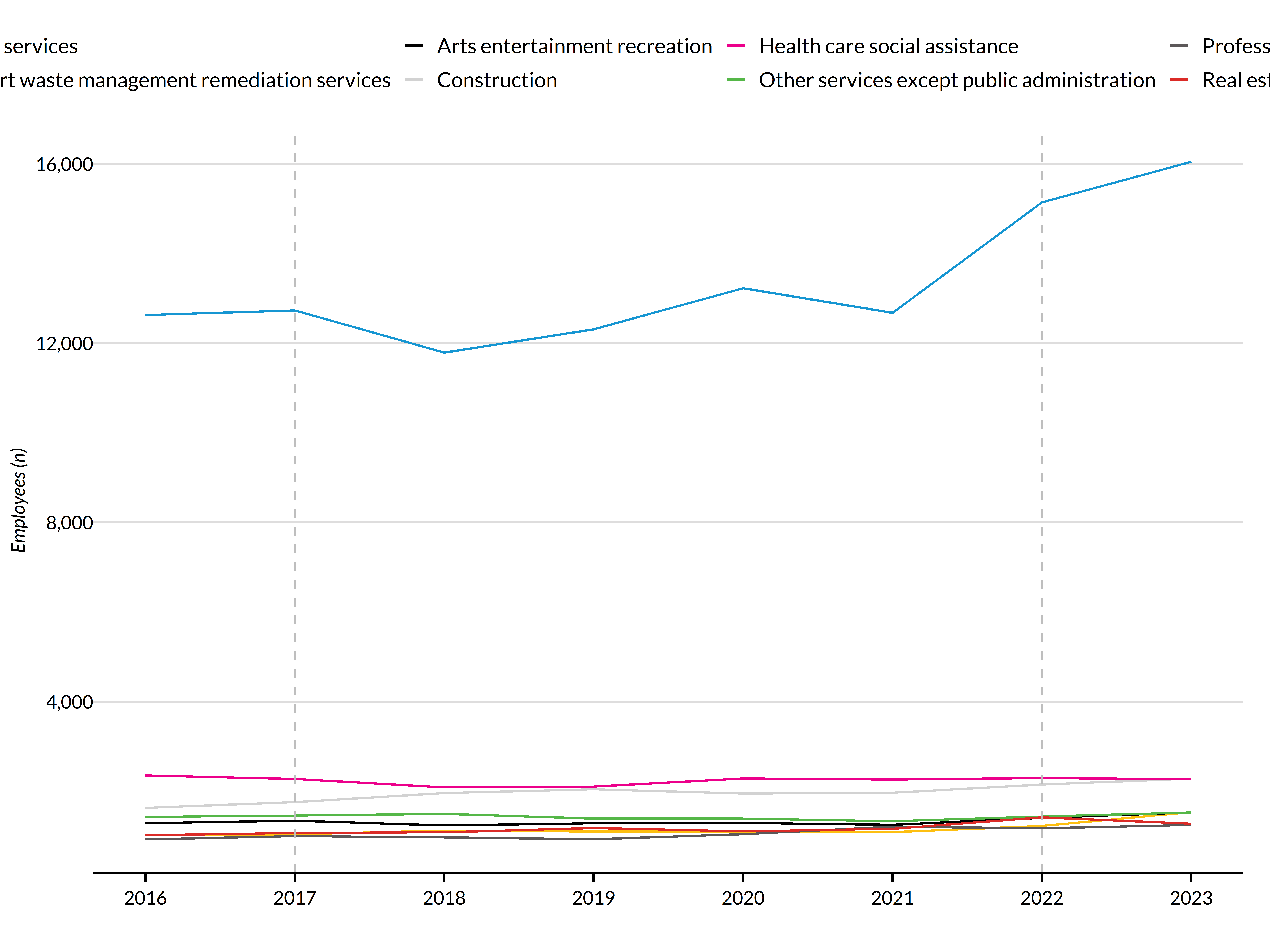

plot of chunk baseline-industry

Small Businesses over Time

Identify smaller businesses, which may be more vulnerable to disaster-related economic shocks.

total_employers = cbp_affected %>%
  filter(industry == "total", employee_size_range_label == "All establishments") %>%
  slice_max(year) %>%
  pull(employers)

cbp_affected %>%
  tibble::as_tibble() %>%
  filter(employee_size_range_label != "All establishments") %>%
  mutate(
    employee_size_range_label = case_when(
      employee_size_range_label %in% c("<100-249 employees", "250-499 employees") ~ "100-499 employees",
      employee_size_range_label %in% c("500-999 employees", "1000+") ~ "500+ employees",
      TRUE ~ employee_size_range_label),
    employee_size_range = factor(
      employee_size_range_label, 
      levels = c(
        "1-4 employees", "<5 employees", "5-9 employees", "10-19 employees", "20-49 employees", 
        "50-99 employees", "100-499 employees", "500+ employees"), 
        ordered = TRUE),
    industry_label = factor(
      industry_label, 
      levels = count(., industry_label, sort = TRUE) %>% pull(industry_label),
      ordered = TRUE)) %>%
  mutate(.by = industry, employer_total = sum(employers)) %>%
  filter(employer_total > (.05 * total_employers)) %>%
  ggplot(aes(x = year)) +
    geom_area(aes(y = employers, fill = employee_size_range)) +
    facet_wrap(~ reorder(industry_label, -employer_total), ncol = 4) +
    labs(x = "Year", y = "Employers", title = "Employers by Number of Employees, by Industry") +
    scale_y_continuous(labels = scales::comma)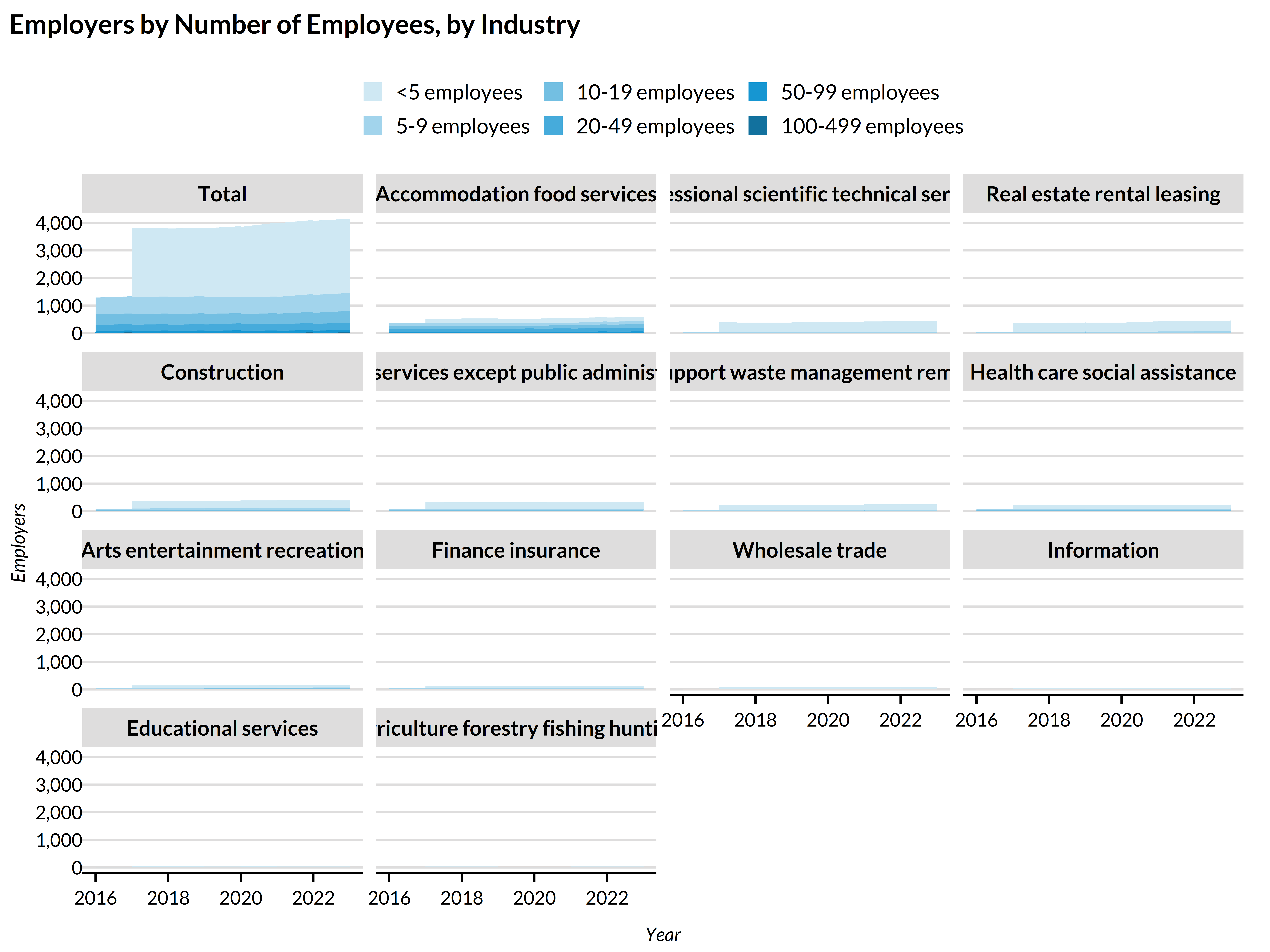

plot of chunk unnamed-chunk-5

County Fiscal Capacity Over Time

county_expenses = get_government_finances()
finances_years = county_expenses %>% pull(year) %>% unique()

finances_prior_disaster_years = disasters_affected %>%
  filter(year_declared %in% finances_years) %>%
  distinct(year_declared)

county_expenses %>%
  filter(GEOID %in% affected_county_fips) %>%
  mutate(across(matches("revenue|expenditure"), ~ .x / 1000)) %>%
  pivot_longer(-c(year, GEOID, county_name)) %>%
  filter(name %in% c("revenue_total", "expenditure_total")) %>%
  mutate(name = if_else(str_detect(name, "expenditure"), "Expenditures", "Revenues")) %>%
  inflation_adjust(year_variable = "year", dollar_variables = "value", base_year = 2024, names_suffix = "_adjusted") %>%
  ggplot(aes(x = year, y = value, color = name, group = name)) +
    geom_line() +
    geom_point() +
    geom_vline(data = finances_prior_disaster_years, color = "grey", linetype = "dashed", aes(xintercept = year_declared)) + 
    scale_y_continuous(labels = scales::dollar_format(suffix = "M")) +
    labs(x = "Year", y = "USD (Millions)")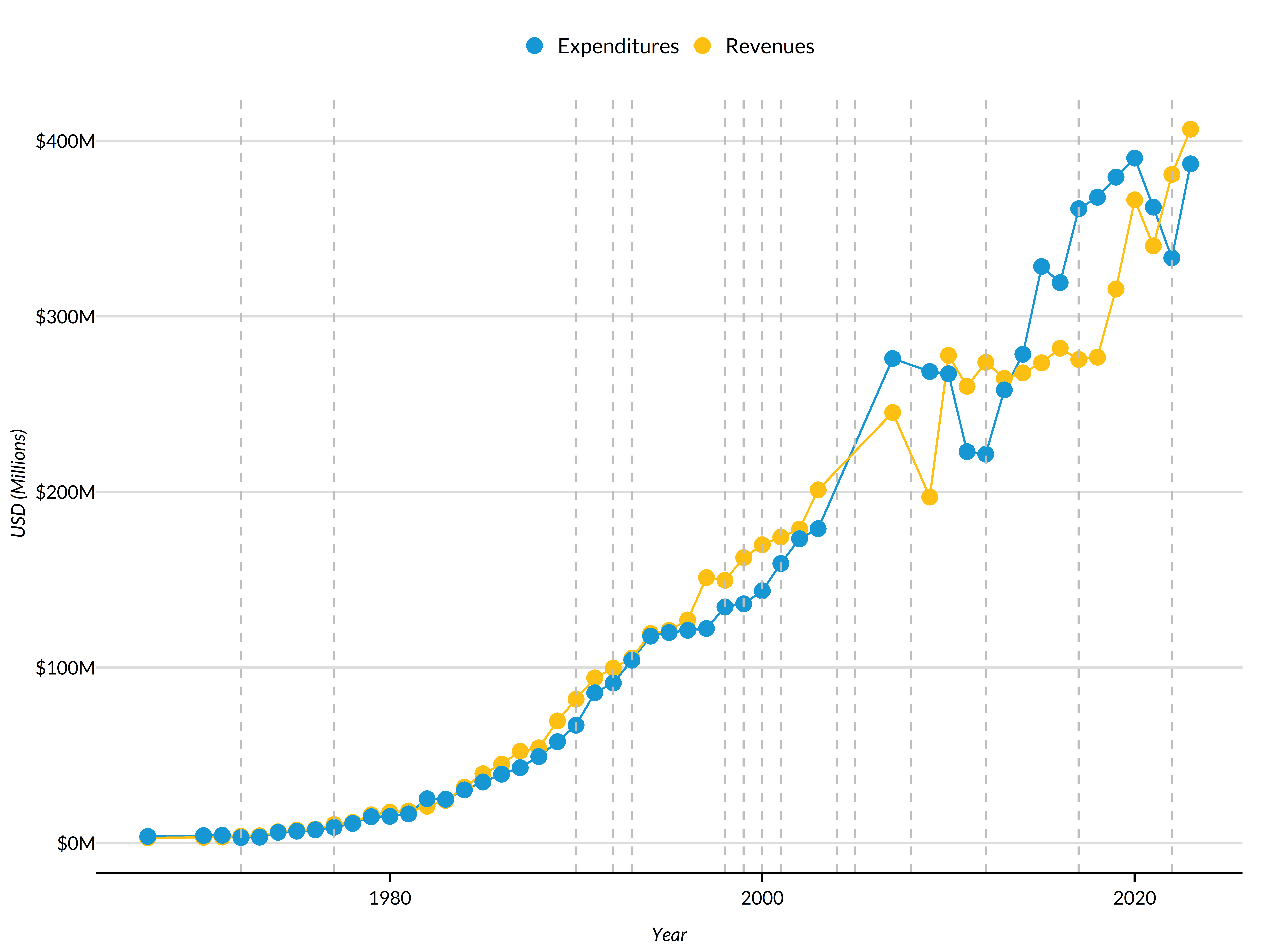 

plot of chunk baseline-fiscal

---

Section 2: Selecting Comparison Counties

Identify historical analogs: counties that experienced similar disasters 5+ years ago.

Assemble Matching Dataset

Build a county-level dataset with all variables needed for matching.

# Disaster history: count and binary indicators by hazard type in past 5 years
disaster_lookback_years <- 5
reference_year <- disaster_year - 1  # Use year before disaster for matching

disaster_history <- disasters %>%
  filter(
    year_declared >= (reference_year - disaster_lookback_years),
    year_declared <= reference_year) %>%
  tidytable::summarise(
    .by = GEOID,
    n_disasters_prior_5yr = sum(incidents_natural_hazard, na.rm = TRUE),
    fire_prior_5yr = as.integer(sum(incidents_fire, na.rm = TRUE) > 0),
    flood_prior_5yr = as.integer(sum(incidents_flood, na.rm = TRUE) > 0),
    hurricane_prior_5yr = as.integer(sum(incidents_hurricane, na.rm = TRUE) > 0),
    severe_storm_prior_5yr = as.integer(sum(incidents_severe_storm, na.rm = TRUE) > 0),
    tornado_prior_5yr = as.integer(sum(incidents_tornado, na.rm = TRUE) > 0),
    winter_storm_prior_5yr = as.integer(sum(incidents_winter_storm, na.rm = TRUE) > 0),
    drought_prior_5yr = as.integer(sum(incidents_drought, na.rm = TRUE) > 0)) %>%
  as_tibble()

sheldus_reference_year = if_else(reference_year < 2023, reference_year, 2023)

sheldus_matching = sheldus_df %>%
  filter(year == sheldus_reference_year)

# Industry employment shares from County Business Patterns
# Use 2-digit NAICS codes for broad sector shares
cbp_reference_year = if_else(reference_year < 2023, reference_year, 2023)

cbp_matching <- cbp_df %>%
  ## filter out the employers by employee size records
  filter(year == cbp_reference_year, employees > 0) %>%
  mutate(GEOID = str_c(state, county)) %>%
  select(GEOID, industry, employees) %>%
  as_tibble()

# Calculate total employment per county
cbp_totals <- cbp_matching %>%
  filter(industry == "total") %>%
  select(GEOID, total_employees = employees)

# Calculate employment share by industry
industry_shares <- cbp_matching %>%
  filter(industry != "total") %>%
  tidylog::left_join(cbp_totals, by = "GEOID") %>%
  arrange(GEOID) %>%
  mutate(
    share_employees_ = employees / total_employees,
    industry_var = str_c("share_employees_", industry)) %>%
  select(GEOID, industry_var, share_employees_) %>%
  pivot_wider(names_from = industry_var, values_from = share_employees_, values_fill = 0)

# Add total employment
## NOTE: the total employee count is always greater than or equal to 
## the sum of individual industries' employment countes because CBP omits
## some industry categories
industry_matching <- industry_shares %>%
  left_join(cbp_totals, by = "GEOID")

# NFIP residential coverage rate by county
nfip_matching <- get_nfip_residential_penetration() %>%
  mutate(share_residential_structures_sfha = residential_structures_sfha / residential_structures) %>%
  select(GEOID, share_residential_structures_sfha, penetration_rate_sfha)

finance_reference_year = if_else(reference_year < 2023, reference_year, 2022)

# Total county government expenses
county_finances_matching = county_expenses %>%
  filter(year == finance_reference_year)

# Sociodemographic characteristics from ACS
acs_matching <- acs_df_2023 %>%
  select(GEOID, all_of(acs_matching_variables))

# Combine all matching variables into single dataset
matching_data <- acs_matching %>%
  left_join(disaster_history, by = "GEOID") %>%
  left_join(sheldus_matching, by = "GEOID") %>%
  left_join(industry_matching, by = "GEOID") %>%
  left_join(nfip_matching, by = "GEOID") %>%
  left_join(county_finances_matching, by = "GEOID") %>%
  # Replace NAs with 0 for disaster counts (counties with no disasters)
  mutate(across(ends_with("_prior_5yr"), ~ replace_na(.x, 0))) %>%
  # Drop counties with missing core variables
  filter(!is.na(total_population_universe), !is.na(total_employees))

Select Comparison Counties

# Hard filter: same disaster type, disaster occurred 5+ years ago
comparison_pool <- disasters %>%
  filter(
    year_declared <= 2021,  # Enough post-period
    year_declared >= 2018) %>%
  slice(.by = GEOID, 1) %>%
  distinct(GEOID, year_declared) %>%
  rename(comparison_disaster_year = year_declared)

# Get affected county's characteristics
affected_county_chars <- matching_data %>%
  filter(GEOID == affected_county_fips)

# Join matching data
comparison_candidates <- comparison_pool %>%
  inner_join(matching_data, by = "GEOID") %>%
  filter(
    total_population_universe > affected_county_chars$total_population_universe * .75,
    total_population_universe < affected_county_chars$total_population_universe * 1.25,
    median_household_income_universe_allraces > affected_county_chars$median_household_income_universe_allraces * .75,
    median_household_income_universe_allraces < affected_county_chars$median_household_income_universe_allraces * 1.25,
    GEOID != affected_county_fips)  # Exclude affected county

# Calculate Mahalanobis distance to affected county

# Select numeric variables for distance calculation
matching_vars <- c(
  acs_matching_variables,
  "n_disasters_prior_5yr",
  "total_employees",
  "penetration_rate_sfha",
  "revenue_total",
  "expenditure_total",
  "damage_property_millions")

# Prepare matrices
matrix_candidates <- comparison_candidates %>%
  select(all_of(matching_vars)) %>%
  as.matrix()

matrix_affected <- affected_county_chars %>%
  select(all_of(matching_vars)) %>%
  as.matrix()

# Calculate covariance matrix and Mahalanobis distance
covariance_matrix <- cov(matrix_candidates, use = "pairwise.complete.obs")
distances <- mahalanobis(matrix_candidates, center = matrix_affected, cov = covariance_matrix, tol=1e-30)

# Select top k nearest neighbors
k_neighbors <- 10

comparison_counties <- comparison_candidates %>%
  mutate(mahalanobis_distance = distances) %>%
  slice_min(mahalanobis_distance, n = k_neighbors) %>%
  select(GEOID, comparison_disaster_year, mahalanobis_distance) %>%
  left_join(tidycensus::fips_codes %>% transmute(county, GEOID = str_c(state_code, county_code))) %>%
  slice(1:5)

---

Section 3: Event-Study Data Preparation

Align all outcome datasets to event time (t=0 is disaster year).

# Create reference table: affected county + comparison counties with disaster years
county_reference <- bind_rows(
  # Affected county
  tibble(
    GEOID = affected_county_fips,
    disaster_year_event = disaster_year,
    county_type = "affected"),
  # Comparison counties
  comparison_counties %>%
    transmute(
      GEOID,
      disaster_year_event = comparison_disaster_year,
      county_type = "comparison"))

# Define event window
event_window <- c(-5, 4)

# Align to event time
cbp_event_aligned <- cbp_df %>%
  mutate(GEOID = str_c(state, county)) %>%
  rename(calendar_year = year) %>%
  inner_join(county_reference, by = "GEOID") %>%
  mutate(event_time = calendar_year - disaster_year_event) %>%
  filter(event_time >= event_window[1], event_time <= event_window[2]) %>%
  select(GEOID, county_type, disaster_year_event, calendar_year, event_time,
         industry, employees, employers, annual_payroll)   

# Align to event time
fiscal_event_aligned <- county_expenses %>%
  rename(calendar_year = year) %>%
  inner_join(county_reference, by = "GEOID") %>%
  mutate(event_time = calendar_year - disaster_year_event) %>%
  filter(event_time >= event_window[1], event_time <= event_window[2]) %>%
  select(GEOID, county_type, disaster_year_event, calendar_year, event_time,
         expenditure_total, revenue_total)

# SBA disaster loans
sba_raw <- get_sba_loans()

sba_crosswalk = get_crosswalk(
  source_geography = "zcta",
  target_geography = "county")

sba_simple = sba_raw %>%
  select(
    source_geoid = damaged_property_zip_code,
    sba_loan_amount = approved_amount_total,
    loan_type,
    fiscal_year)

warning("The crosswalking is imperfect and fiscal and calendar years are not aligned.")
sba_county = sba_simple %>%
  tidylog::left_join(sba_crosswalk$crosswalks$step_1, by = "source_geoid") %>%
  mutate(target_geoid = str_c(state_fips, target_geoid)) %>%
  tidytable::summarize(
    .by = c(target_geoid, loan_type, fiscal_year),
    sba_loan_amount = sum(sba_loan_amount * allocation_factor_source_to_target)) %>%
  filter(!is.na(target_geoid)) %>%
  mutate(
    GEOID = target_geoid, 
    calendar_year = fiscal_year %>% as.numeric) %>%
  pivot_wider(names_from = loan_type, values_from = sba_loan_amount) %>%
  rename(business_loan = business, residential_loan = residential) %>%
  mutate(across(matches("loan"), ~ if_else(is.na(.x), 0, .x)))

# Align to event time
sba_event_aligned <- sba_county %>%
  inner_join(county_reference, by = "GEOID") %>%
  mutate(event_time = calendar_year - disaster_year_event) %>%
  filter(event_time >= event_window[1], event_time <= event_window[2]) %>%
  select(GEOID, county_type, disaster_year_event, calendar_year, event_time,
         matches("loan"))

# FEMA Public Assistance
pa_raw <- get_public_assistance()
#> 
Processed 360244 groups out of 656351. 55% done. Time elapsed: 3s. ETA: 2s.
Processed 550614 groups out of 656351. 84% done. Time elapsed: 4s. ETA: 0s.
Processed 656351 groups out of 656351. 100% done. Time elapsed: 4s. ETA: 0s.

# Aggregate to county-year level
pa_county_year <- pa_raw %>%
  mutate(
    GEOID = county_fips,
    calendar_year = declaration_year) %>%
  summarise(
    .by = c(GEOID, calendar_year),
    across(.cols = matches("split"), ~ sum(.x, na.rm = TRUE)))

# Align to event time
pa_event_aligned <- pa_county_year %>%
  inner_join(county_reference, by = "GEOID") %>%
  mutate(event_time = calendar_year - disaster_year_event) %>%
  filter(event_time >= event_window[1], event_time <= event_window[2]) %>%
  select(GEOID, county_type, disaster_year_event, calendar_year, event_time,
         pa_federal_funding_obligated_split)

# FEMA Individual and Households Program
# ihp_raw <- get_ihp_registrations()

# # Aggregate to county-year level
# ihp_county_year <- ihp_raw %>%
#   mutate(calendar_year = lubridate::year(declaration_date)) %>%
#   summarise(
#     .by = c(GEOID, calendar_year),
#     ihp_registrations_n = n(),
#     ihp_approved_n = sum(ihp_eligible, na.rm = TRUE),
#     ihp_amount_total = sum(ihp_amount, na.rm = TRUE),
#     ihp_ha_amount = sum(ha_amount, na.rm = TRUE),
#     ihp_ona_amount = sum(ona_amount, na.rm = TRUE))

# # Align to event time
# ihp_event_aligned <- ihp_county_year %>%
#   inner_join(county_reference, by = "GEOID") %>%
#   mutate(event_time = calendar_year - disaster_year_event) %>%
#   filter(event_time >= event_window[1], event_time <= event_window[2]) %>%
#   select(GEOID, county_type, disaster_year_event, calendar_year, event_time,
#          ihp_registrations_n, ihp_approved_n, ihp_amount_total, ihp_ha_amount, ihp_ona_amount)

---

Section 4: Employment Trajectories (Event-Study Style)

Plot employment trends with time relative to disaster (t=0).

• Affected county: t-6 through t=0 (present)
• Comparison counties: full t-6 through t+6 window, aligned to their disaster year

# Total employment over event time
cbp_event_aligned %>%
  filter(industry == "total", employees > 0) %>%
  tibble::as_tibble() %>%
  ggplot(aes(x = event_time, y = employees, group = GEOID, color = county_type, linetype = county_type)) +
  geom_line() +
  geom_point() +
  ylim(c(0, NA)) +
  geom_vline(xintercept = 0, linetype = "dashed", color = "grey40") +
  scale_y_continuous(labels = scales::comma) +
  scale_color_manual(values = c("affected" = "#1696d2", "comparison" = "#d2d2d2")) +
  labs(
    x = "Years Relative to Disaster (t=0)",
    y = "Total Employees",
    title = "Employment Trajectory: Affected vs. Comparison Counties") +
  theme(legend.position = "none")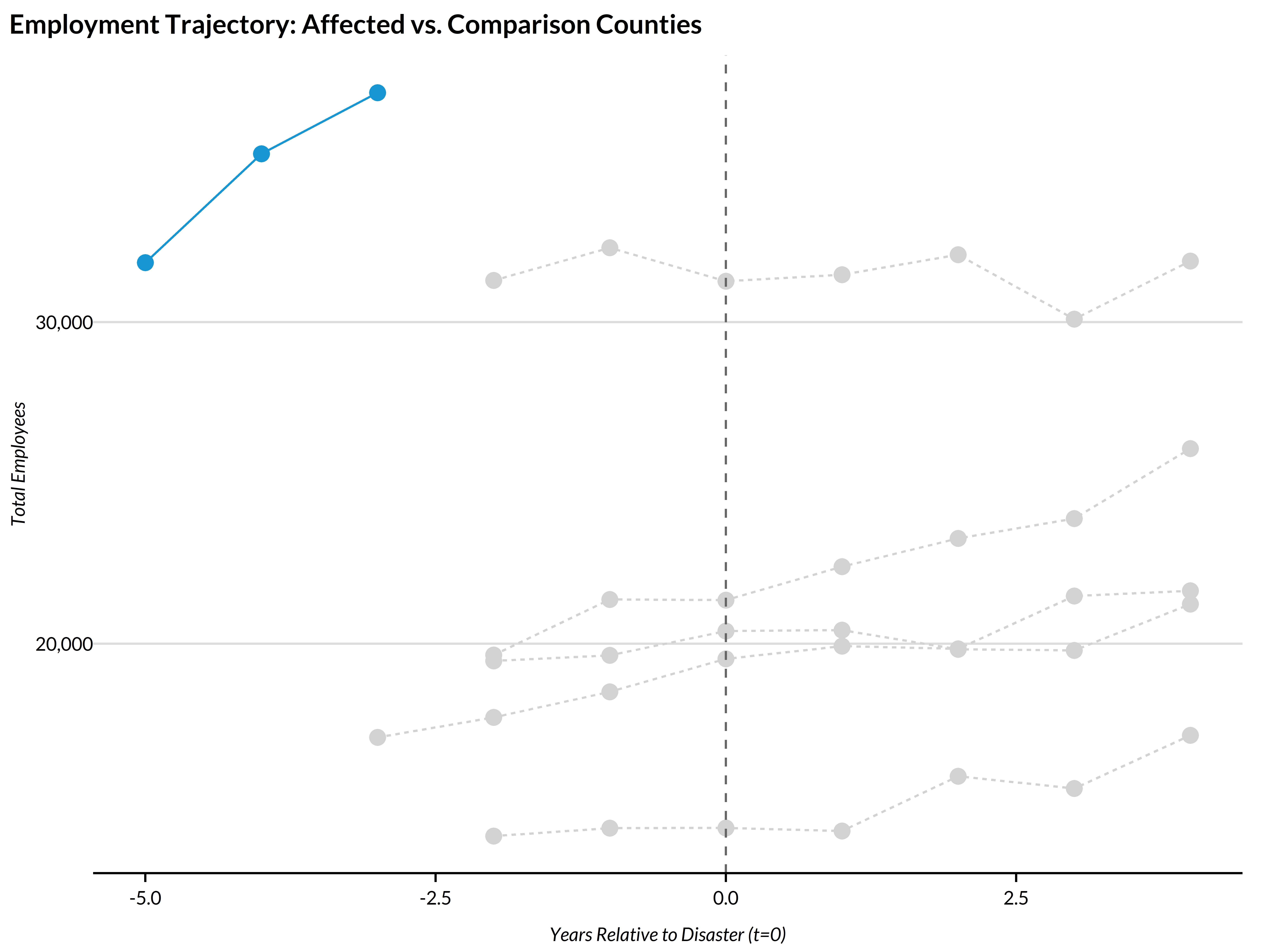

plot of chunk employment-total

---

Section 5: Local Government Fiscal Trajectories (Event-Study Style)

Examine how local government finances evolved in comparison counties post-disaster.

# Total county expenses over event time
fiscal_event_aligned %>%
  mutate(county_type = if_else(str_detect(county_type, "affected"), "Impacted", "Comparison")) %>%
  ggplot(aes(x = event_time, y = expenditure_total / 1000, group = GEOID, color = county_type)) +
  geom_line() +
  geom_point() +
  geom_vline(xintercept = 0, linetype = "dashed", color = "grey40") +
  scale_y_continuous(labels = scales::dollar_format(suffix = "M")) +
  ylim(c(0, NA)) +
  scale_color_manual(values = c("Impacted" = "#1696d2", "Comparison" = "#d2d2d2")) +
  labs(
    x = "Years Relative to Disaster (t=0)",
    y = "Total County Expenses (Millions)",
    title = "County Government Expenses: Affected vs. Comparison Counties") +
  theme(legend.position = "none")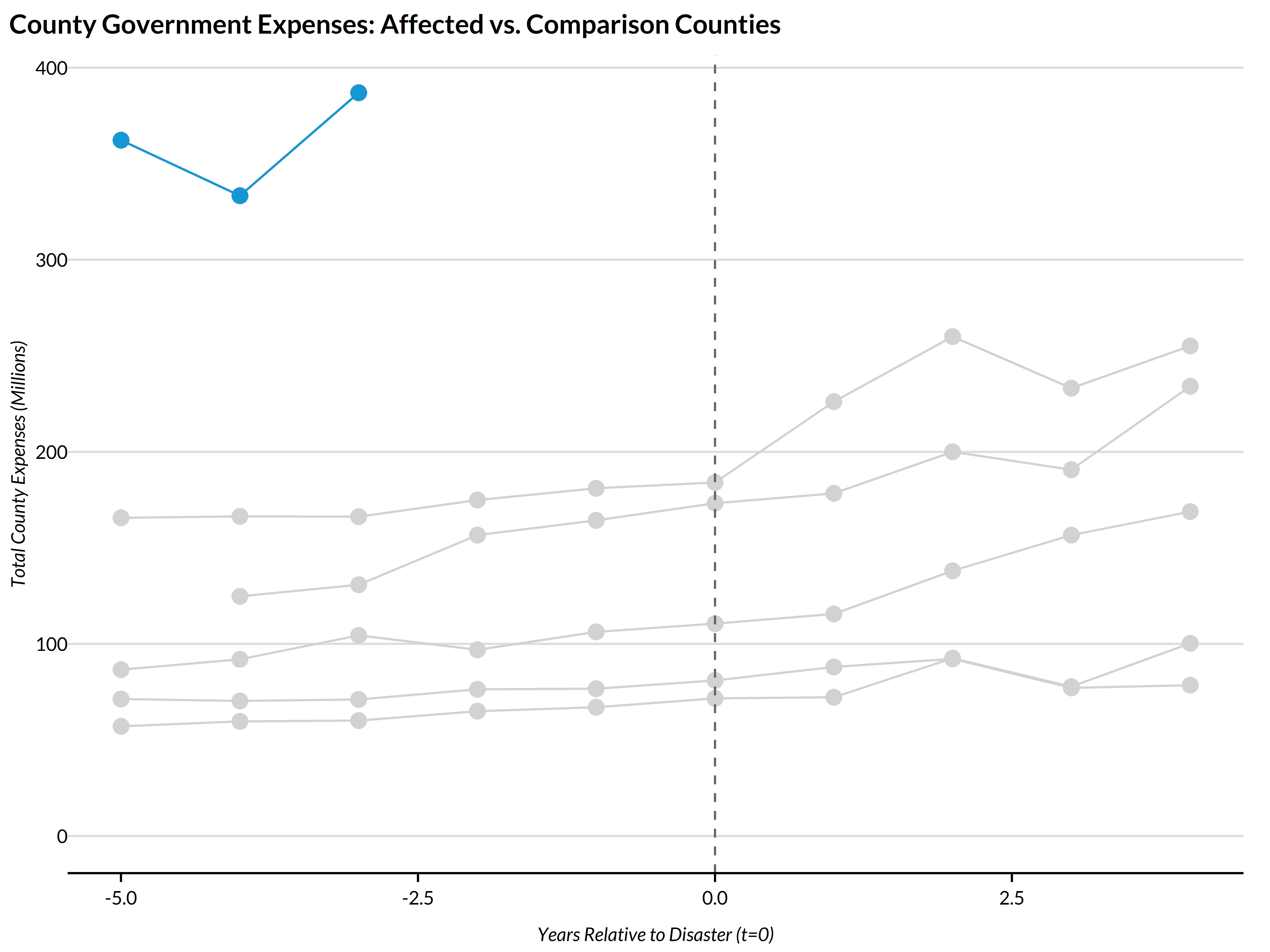

plot of chunk fiscal-expenses

# Total county expenses over event time
fiscal_event_aligned %>%
  mutate(county_type = if_else(str_detect(county_type, "affected"), "Impacted", "Comparison")) %>%
  ggplot(aes(x = event_time, y = revenue_total / 1000, group = GEOID, color = county_type)) +
  geom_line() +
  geom_point() +
  geom_vline(xintercept = 0, linetype = "dashed", color = "grey40") +
  scale_y_continuous(labels = scales::dollar_format(suffix = "M")) +
  scale_color_manual(values = c("Impacted" = "#1696d2", "Comparison" = "#d2d2d2")) +
  labs(
    x = "Years Relative to Disaster (t=0)",
    y = "Total County Revenues (Millions)",
    title = "County Government Revenues: Affected vs. Comparison Counties") +
  theme(legend.position = "none")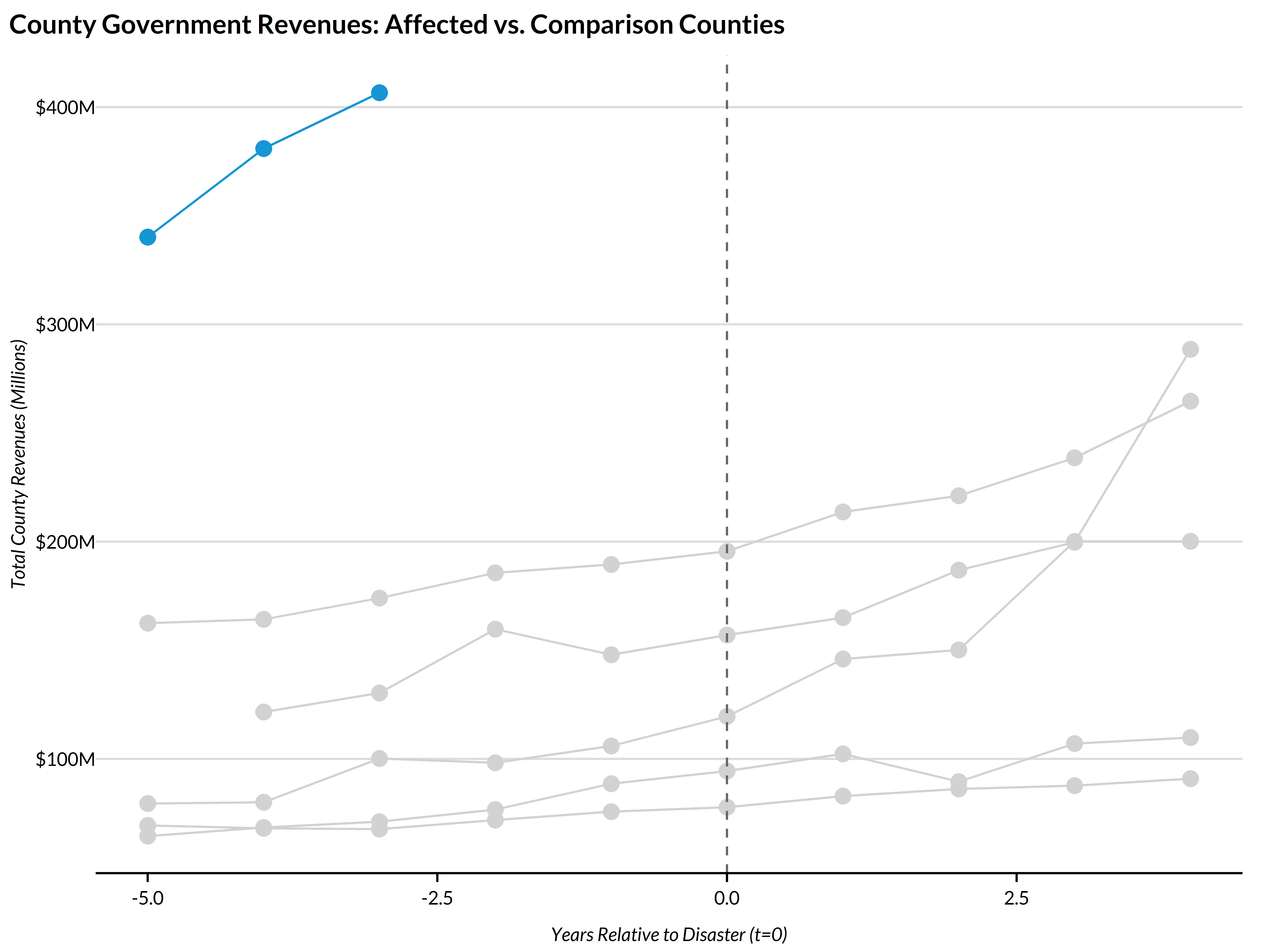

plot of chunk fiscal-revenue

---

Section 6: Recovery Resources in Comparison Cases

Describe typical federal assistance flows based on historical analogs. Since the affected county’s disaster just occurred, we show comparison counties’ post-disaster resource flows as projections.

SBA Disaster Loans

# SBA loans over event time (comparison counties only for post-period)

sba_event_aligned %>%
  arrange(GEOID, event_time) %>%
  mutate(
    .by = GEOID,
    across(matches("loan"), ~ cumsum(.x))) %>%
  mutate(county_type = if_else(str_detect(county_type, "affected"), "Impacted", "Comparison")) %>%
  ggplot(aes(x = event_time, y = residential_loan / 1000000, group = GEOID, color = county_type)) +
  geom_line() +
  ylim(c(0, NA)) +
  geom_vline(xintercept = 0, linetype = "dashed", color = "grey40") +
  scale_y_continuous(labels = scales::dollar_format(suffix = "M")) +
  scale_color_manual(values = c("Impacted" = "#1696d2", "Comparison" = "#d2d2d2")) +
  labs(
    x = "Years relative to disaster (t=0)",
    y = "SBA loans (cumulative)",
    title = "Cumulative SBA Loans - Residential") +
  theme(legend.position = "none")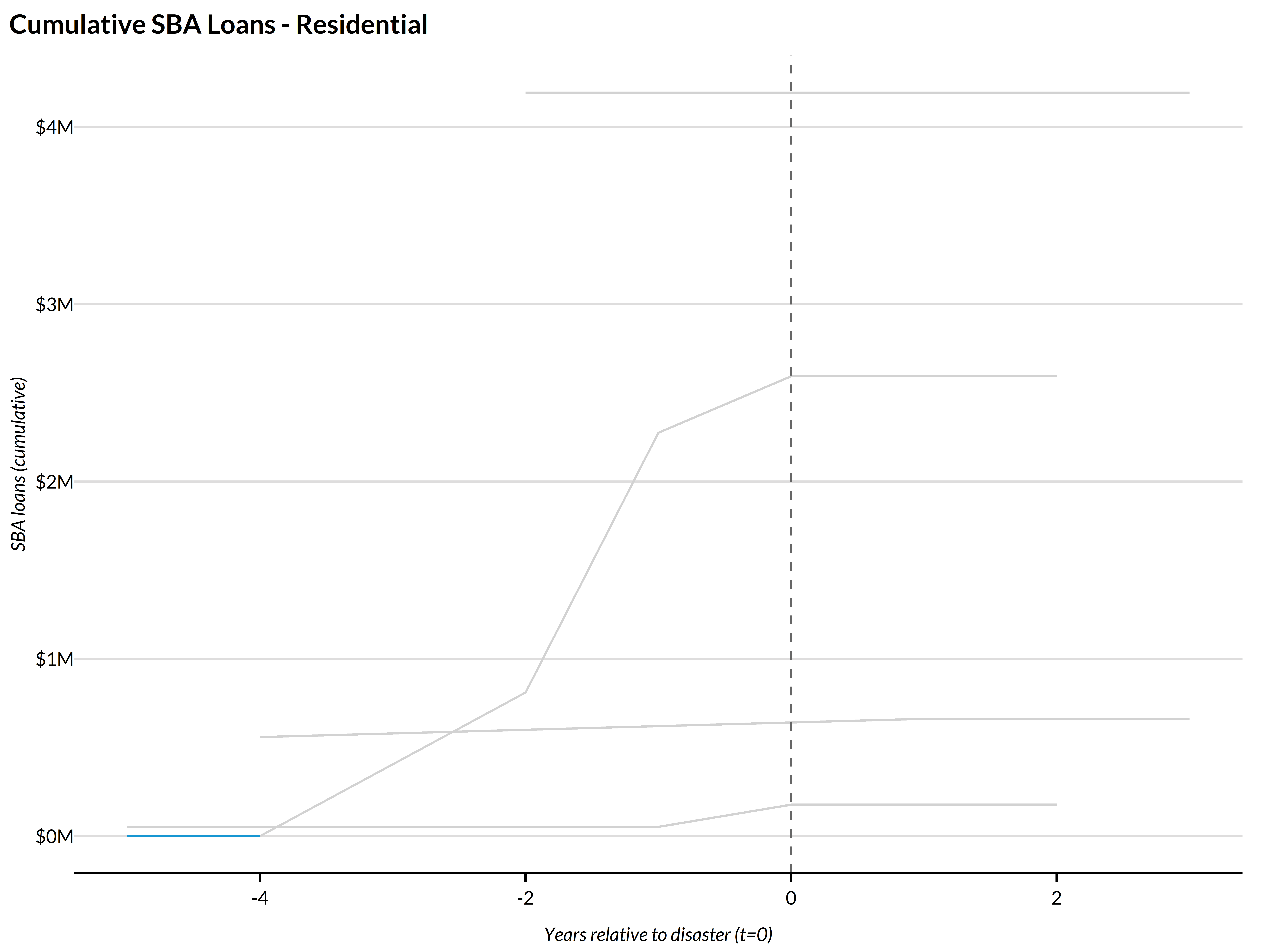

plot of chunk recovery-sba

sba_event_aligned %>%
  arrange(GEOID, event_time) %>%
  mutate(
    .by = GEOID,
    across(matches("loan"), ~ cumsum(.x))) %>%
  ggplot(aes(x = event_time, y = business_loan / 1000000, group = GEOID, color = county_type)) +
  geom_line() +
  geom_vline(xintercept = 0, linetype = "dashed", color = "grey40") +
  scale_y_continuous(labels = scales::dollar_format(suffix = "M")) +
  scale_color_manual(values = c("affected" = "#1696d2", "comparison" = "#d2d2d2")) +
  labs(
    x = "Years relative to disaster (t=0)",
    y = "SBA loans (cumulative)",
    title = "Cumulative SBA Loans - Business") +
  theme(legend.position = "none")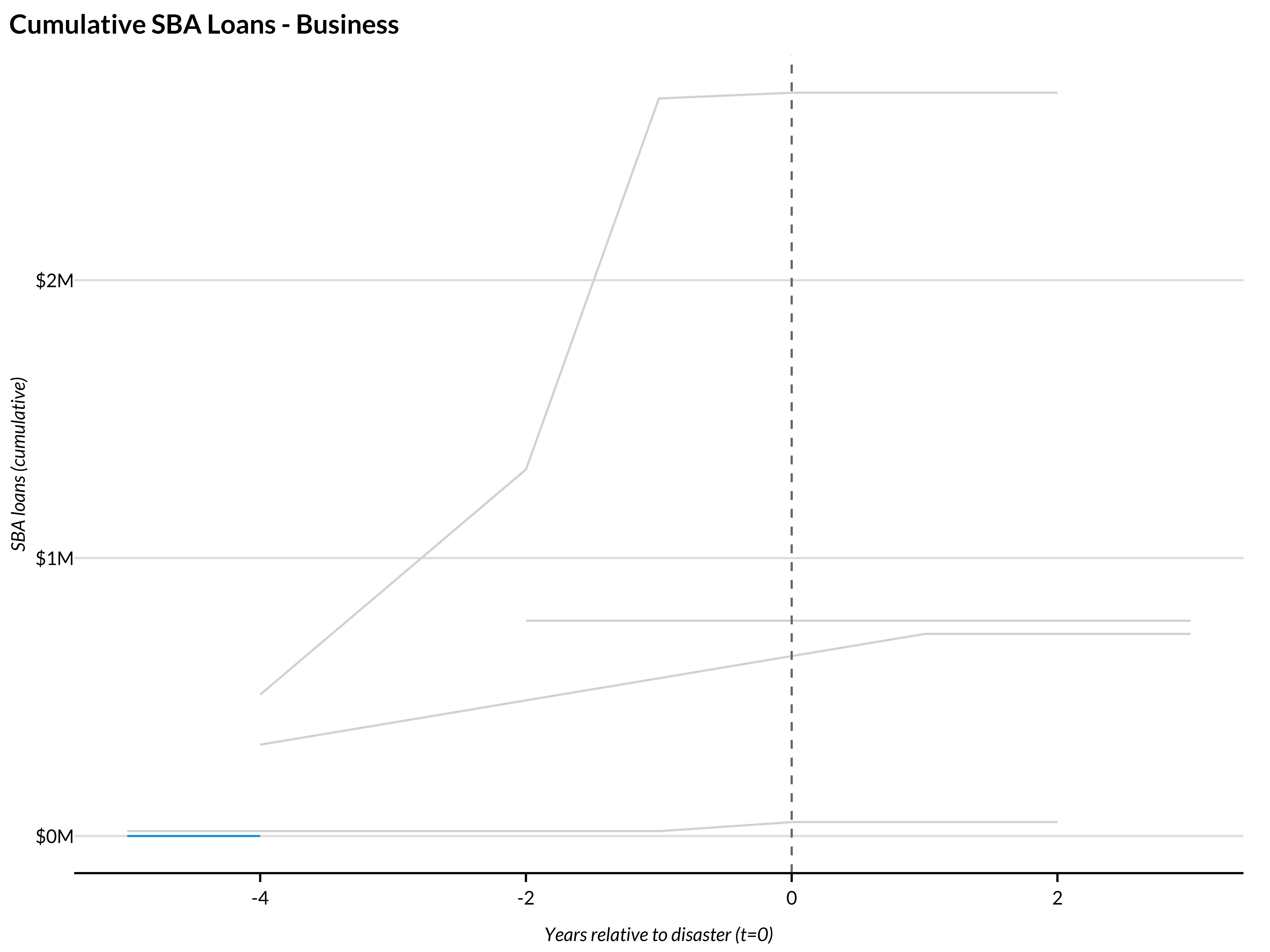

plot of chunk recovery-sba

FEMA Public Assistance

# PA funding over event time (comparison counties only for post-period)
pa_event_aligned %>%
  mutate(county_type = if_else(str_detect(county_type, "affected"), "Impacted", "Comparison")) %>%
  ggplot(aes(x = event_time, y = pa_federal_funding_obligated_split / 1e6, group = GEOID, color = county_type)) +
  geom_line() +
  geom_vline(xintercept = 0, linetype = "dashed", color = "grey40") +
  scale_y_continuous(labels = scales::dollar_format(suffix = "M")) +
  scale_color_manual(values = c("Impacted" = "#1696d2", "Comparison" = "#d2d2d2")) +
  labs(
    x = "Years Relative to Disaster (t=0)",
    y = "FEMA PA Federal Share Obligated (Millions)",
    title = "FEMA Public Assistance in Comparison Counties")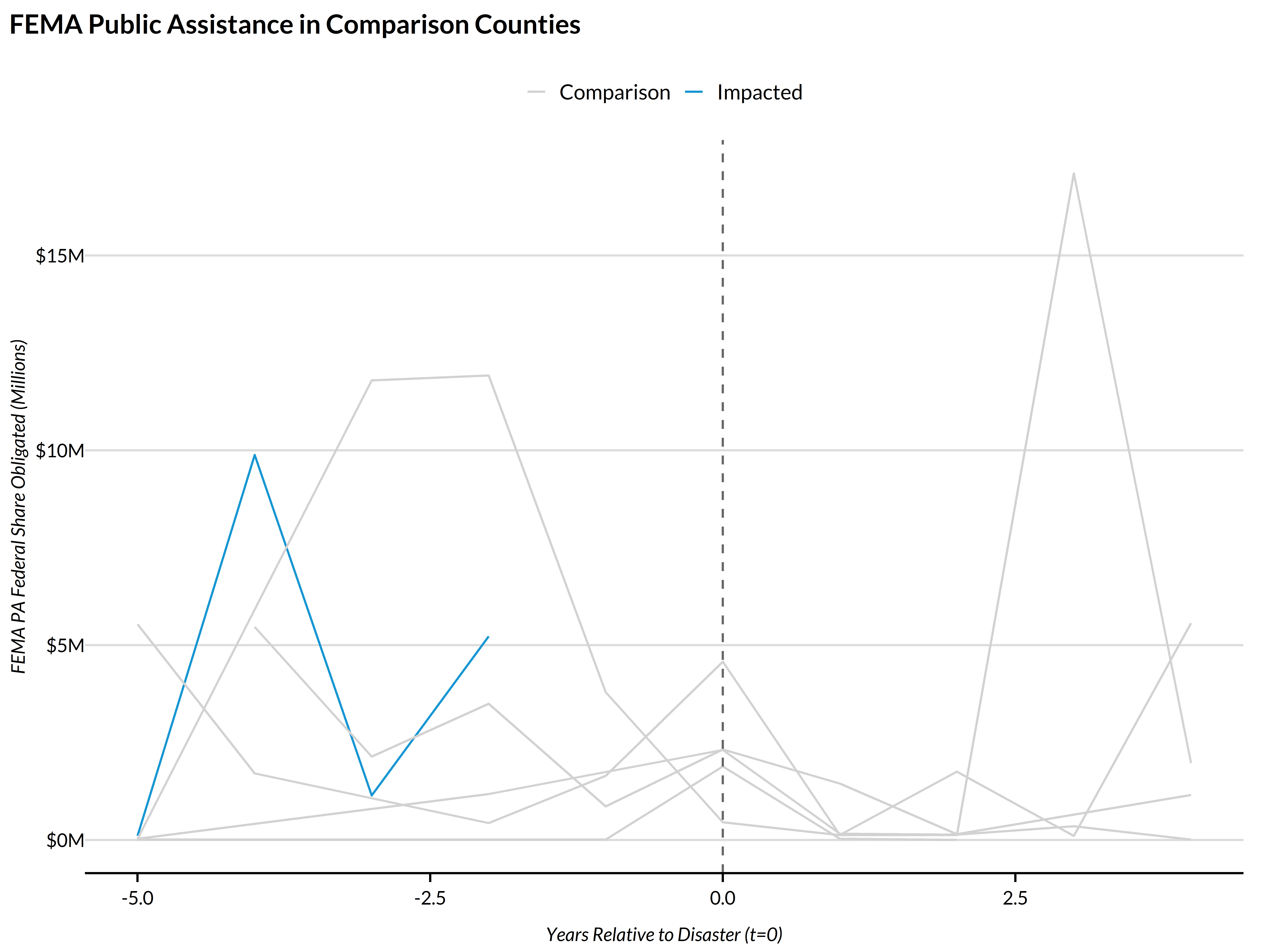

plot of chunk recovery-pa

Individual and Households Program

# # IHP funding over event time (comparison counties only for post-period)
# ihp_event_aligned %>%
#   ggplot(aes(x = event_time, y = ihp_amount_total / 1e6, group = GEOID)) +
#   geom_line(alpha = 0.4, color = "#d2d2d2") +
#   stat_summary(aes(group = 1), fun = median, geom = "line", color = "#1696d2", linewidth = 1.2) +
#   geom_vline(xintercept = 0, linetype = "dashed", color = "grey40") +
#   scale_y_continuous(labels = scales::dollar_format(suffix = "M")) +
#   labs(
#     x = "Years Relative to Disaster (t=0)",
#     y = "IHP Total Amount (Millions)",
#     title = "FEMA Individual & Households Program in Comparison Counties",
#     subtitle = "Blue line = median across comparison counties"
#   )

---

Section 7: Key Takeaways

# Programmatically generate summary statistics for the factsheet:
# - Pre-disaster vulnerability indicators for affected county
# - Median/range of recovery trajectories from comparison counties
# - Typical federal resource flows

Summary Table

# Create summary table of key indicators

---

Technical Notes

Comparison County Selection Criteria

• Similar population size and income (within 25% of affected county in either direction)

Data Availability Notes

• LODES data typically lag 2 years
• County Business Patterns lag 2 years
• Government finances lag 2
• FEMA assistance data are near real-time