SHELDUS Hazard Data

Overview

The get_sheldus() function provides access to county-level hazard event data from the Spatial Hazard Events and Losses Database for the United States (SHELDUS). This database tracks property damage, crop damage, fatalities, and injuries from natural hazards across all US counties.

Data source

SHELDUS is maintained by Arizona State University’s Center for Emergency Management and Homeland Security. The database compiles hazard event data from multiple sources including NOAA Storm Events, the National Climatic Data Center, and other federal agencies.

Access to SHELDUS requires a subscription. See https://cemhs.asu.edu/sheldus for more information.

Loading the data

library(climateapi)
library(tidyverse)
library(sf)
library(urbnthemes)

set_urbn_defaults(style = "print")

sheldus <- get_sheldus()

Data structure

Each row represents a unique combination of county, year, month, and hazard type. Only county-month-hazard combinations with recorded events are included.

glimpse(sheldus)
#> Rows: 1,000,189
#> Columns: 13
#> $ unique_id         <chr> "199da95a-821f-4f2f-974a-85bb0c4e8a0f", "a9af66c4-1ea9-4c43-9a7e-85211bf280db", "b6e481a5-998b-46a3-a393-0064de9e87b4", "e40fd03d-cabf-4e41-9…
#> $ GEOID             <chr> "01001", "01001", "01001", "01001", "01001", "01001", "01001", "01001", "01001", "01001", "01001", "01001", "01001", "01001", "01001", "01001…
#> $ state_name        <chr> "Alabama", "Alabama", "Alabama", "Alabama", "Alabama", "Alabama", "Alabama", "Alabama", "Alabama", "Alabama", "Alabama", "Alabama", "Alabama"…
#> $ county_name       <chr> "Autauga", "Autauga", "Autauga", "Autauga", "Autauga", "Autauga", "Autauga", "Autauga", "Autauga", "Autauga", "Autauga", "Autauga", "Autauga"…
#> $ year              <dbl> 1961, 1961, 1961, 1962, 1962, 1962, 1962, 1962, 1963, 1963, 1963, 1964, 1964, 1965, 1966, 1967, 1968, 1968, 1968, 1969, 1969, 1969, 1969, 196…
#> $ month             <dbl> 1, 2, 12, 1, 4, 4, 4, 12, 1, 4, 12, 4, 4, 7, 1, 3, 3, 8, 8, 3, 3, 6, 6, 6, 4, 4, 4, 5, 1, 3, 3, 4, 4, 4, 5, 5, 5, 6, 3, 3, 2, 4, 5, 11, 1, 2,…
#> $ hazard            <chr> "Winter Weather", "Severe Storm/Thunder Storm", "Severe Storm/Thunder Storm", "Winter Weather", "Hail", "Severe Storm/Thunder Storm", "Wind",…
#> $ damage_property   <dbl> 21498.713, 75141.081, 83907.468, 74394.646, 2479.825, 2479.825, 2479.825, 74394.646, 73422.069, 491928.296, 73422.167, 292024.963, 6389.224, …
#> $ damage_crop       <dbl> 7514.11815, 75141.08081, 8390.71660, 74394.64644, 2479.82487, 2479.82487, 2479.82487, 74394.64644, 73422.06910, 0.00000, 7342.22659, 34952.83…
#> $ fatalities        <dbl> 0.00, 0.00, 0.00, 0.06, 0.00, 0.00, 0.00, 0.04, 0.00, 0.00, 0.00, 0.00, 0.00, 1.00, 0.15, 0.00, 0.00, 0.00, 0.00, 0.00, 0.00, 0.00, 0.00, 0.0…
#> $ injuries          <dbl> 0.00000, 0.00000, 0.00000, 0.00000, 0.00333, 0.00333, 0.00333, 0.00000, 0.00000, 0.00000, 0.00000, 0.04000, 0.04000, 0.00000, 0.07000, 0.0000…
#> $ records           <dbl> 2, 1, 1, 1, 1, 1, 1, 1, 1, 1, 1, 2, 1, 1, 1, 1, 1, 1, 1, 1, 1, 1, 1, 1, 1, 1, 1, 1, 1, 2, 2, 1, 1, 1, 1, 1, 1, 1, 1, 2, 1, 1, 1, 1, 1, 1, 1, …
#> $ allocation_factor <dbl> NA, NA, NA, NA, NA, NA, NA, NA, NA, NA, NA, NA, NA, NA, NA, NA, NA, NA, NA, NA, NA, NA, NA, NA, NA, NA, NA, NA, NA, NA, NA, NA, NA, NA, NA, N…

Key variables include:

unique_id: Unique identifier for each observation
GEOID: Five-digit county FIPS code
year and month: Temporal identifiers
hazard: Type of hazard event (e.g., “Flooding”, “Hurricane/Tropical Storm”)
damage_property: Property damage in 2023 inflation-adjusted dollars
damage_crop: Crop damage in 2023 inflation-adjusted dollars
fatalities and injuries: Human impacts
records: Number of individual events aggregated into the observation

Example analyses

Hazard types in the database

sheldus |>
  distinct(hazard) |>
  arrange(hazard) |>
  pull(hazard)
#>  [1] "Avalanche"                  "Coastal"                    "Drought"                    "Earthquake"                 "Flooding"                  
#>  [6] "Fog"                        "Hail"                       "Heat"                       "Hurricane/Tropical Storm"   "Landslide"                 
#> [11] "Lightning"                  "Severe Storm/Thunder Storm" "Tornado"                    "Tsunami/Seiche"             "Volcano"                   
#> [16] "Wildfire"                   "Wind"                       "Winter Weather"

Annual property damage by hazard type

df1 <- sheldus |>
  summarize(
    .by = c(year, hazard),
    total_damage = sum(damage_property, na.rm = TRUE) / 1e9)

top_hazards <- df1 |>
  summarize(
    .by = hazard,
    total = sum(total_damage, na.rm = TRUE)) |>
  slice_max(total, n = 5) |>
  pull(hazard)

df1 |>
  filter(hazard %in% top_hazards) |>
  ggplot(aes(x = year, y = total_damage, fill = hazard)) +
  geom_col() +
  scale_fill_manual(values = c(
    palette_urbn_main[1:4], palette_urbn_cyan[5])) +
  labs(
    title = "Annual Property Damage by Hazard Type",
    subtitle = "Top 5 hazard types by total damage, 2023 dollars",
    x = "",
    y = "Property damage (billions)",
    fill = "Hazard type")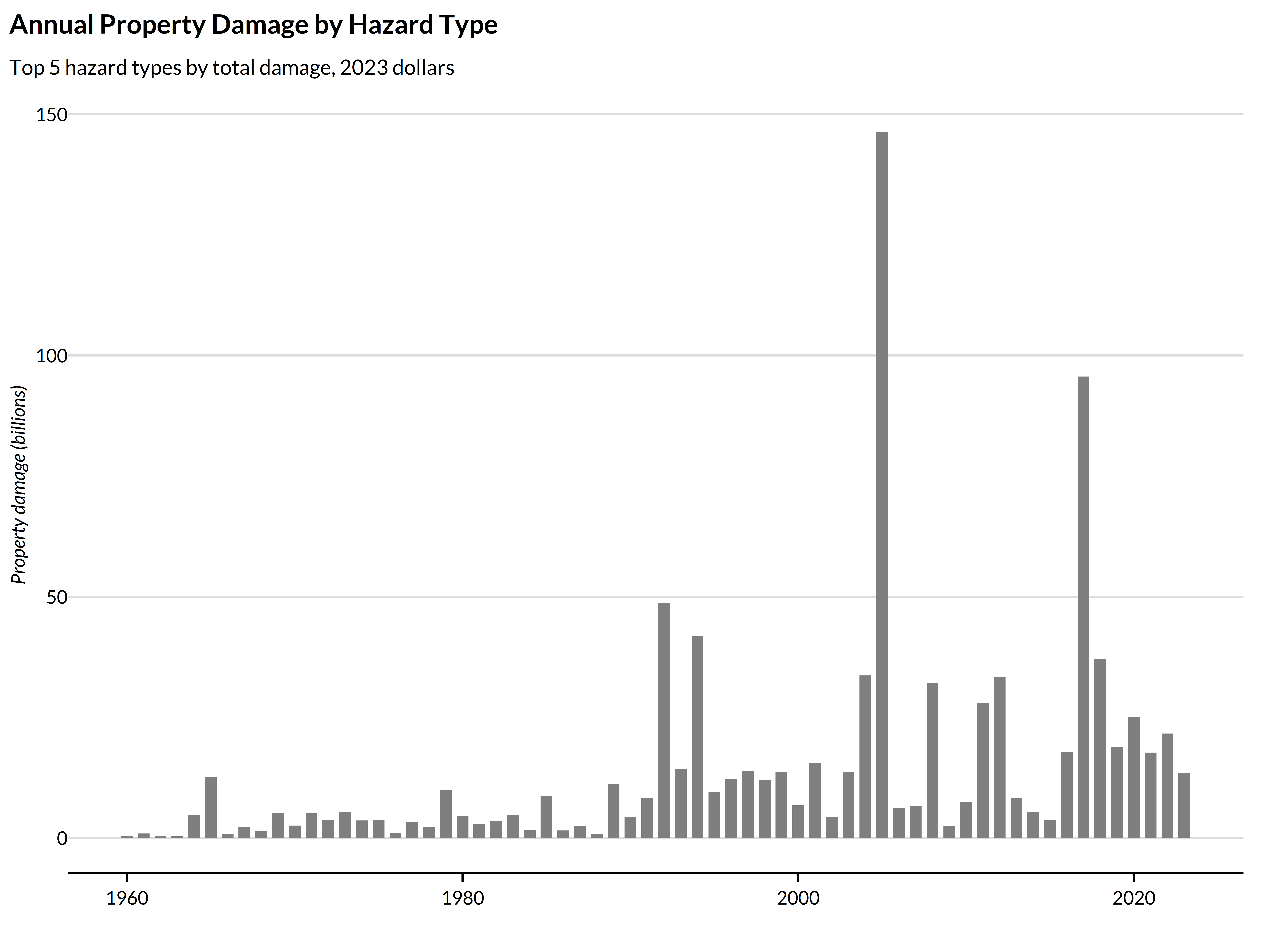

plot of chunk annual-damage

Geographic distribution of flood damage

flood_damage <- sheldus |>
  filter(hazard == "Flooding") |>
  summarize(
    .by = GEOID,
    total_damage = sum(damage_property, na.rm = TRUE))

counties_sf <- tigris::counties(cb = TRUE, year = 2022, progress_bar = FALSE) |>
  st_transform(5070) |>
  filter(!STATEFP %in% c("02", "15", "72", "78", "66", "60", "69"))

flood_map <- counties_sf |>
  left_join(flood_damage, by = "GEOID") |>
  mutate(
    damage_category = case_when(
      is.na(total_damage) | total_damage == 0 ~ "No recorded damage",
      total_damage < 1e6 ~ "< $1M",
      total_damage < 10e6 ~ "$1M - $10M",
      total_damage < 100e6 ~ "$10M - $100M",
      TRUE ~ "> $100M"),
    damage_category = factor(
      damage_category,
      levels = c("No recorded damage", "< $1M", "$1M - $10M", "$10M - $100M", "> $100M")))

ggplot(flood_map) +
  geom_sf(aes(fill = damage_category), color = NA) +
  scale_fill_manual(values = c(
    "No recorded damage" = "grey90",
    "< $1M" = palette_urbn_cyan[1],
    "$1M - $10M" = palette_urbn_cyan[3],
    "$10M - $100M" = palette_urbn_cyan[5],
    "> $100M" = palette_urbn_cyan[7])) +
  labs(
    title = "Cumulative Flood Damage by County",
    subtitle = "Total property damage from flooding events, 2023 dollars",
    fill = "Total damage") +
  theme_urbn_map()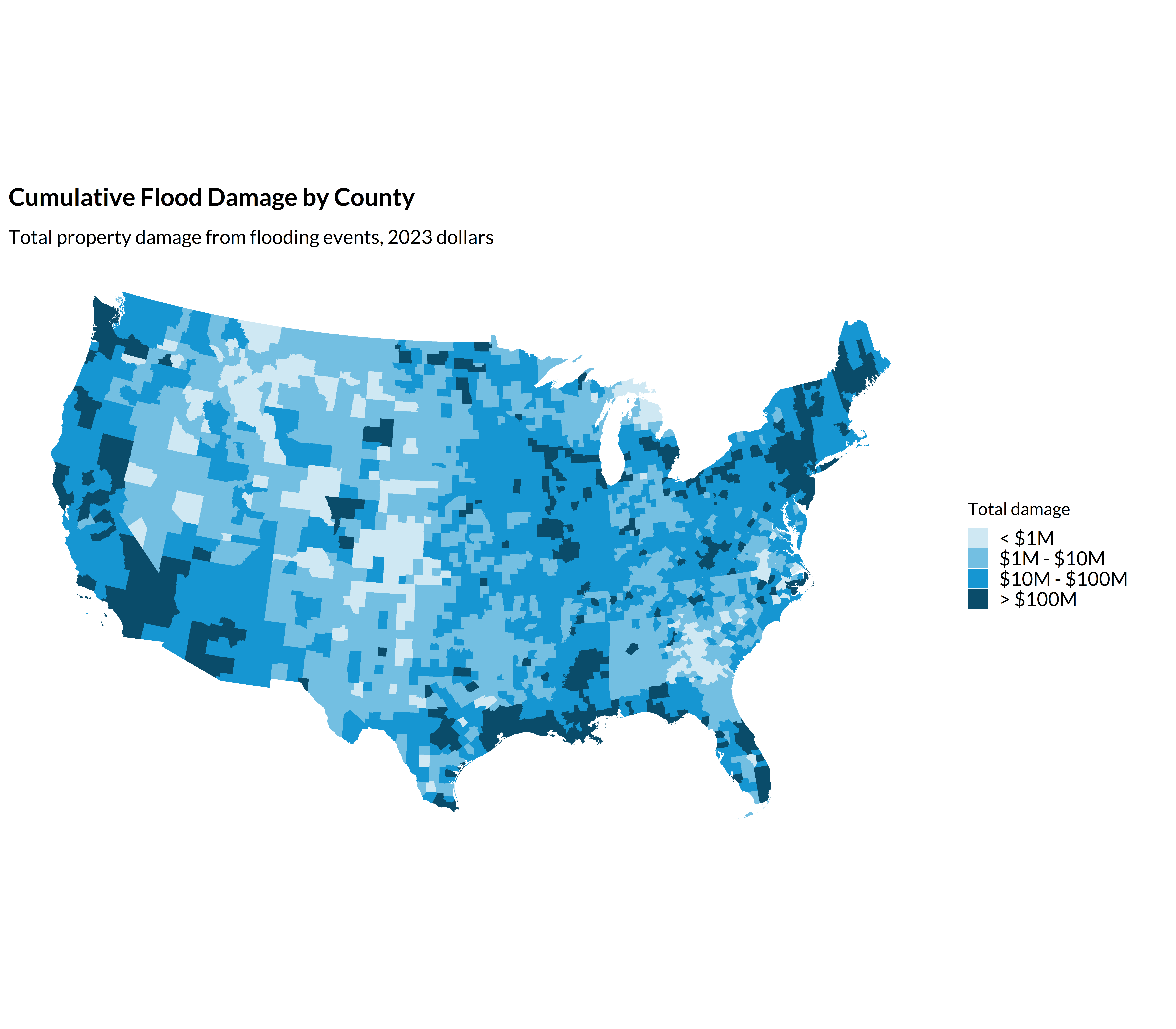

plot of chunk flood-damage-map

Seasonal patterns in hazard events

seasonal <- sheldus |>
  filter(hazard %in% top_hazards) |>
  summarize(
    .by = c(month, hazard),
    total_events = sum(records, na.rm = TRUE))

ggplot(seasonal, aes(x = month, y = total_events, color = hazard)) +
  geom_line(linewidth = 1) +
  geom_point(size = 2) +
  scale_x_continuous(breaks = 1:12, labels = month.abb) +
  scale_color_manual(values = c(
    palette_urbn_main[1:4], palette_urbn_cyan[5])) +
  labs(
    title = "Seasonal Distribution of Hazard Events",
    subtitle = "Total event count by month across all years",
    x = "",
    y = "Number of events",
    color = "Hazard type")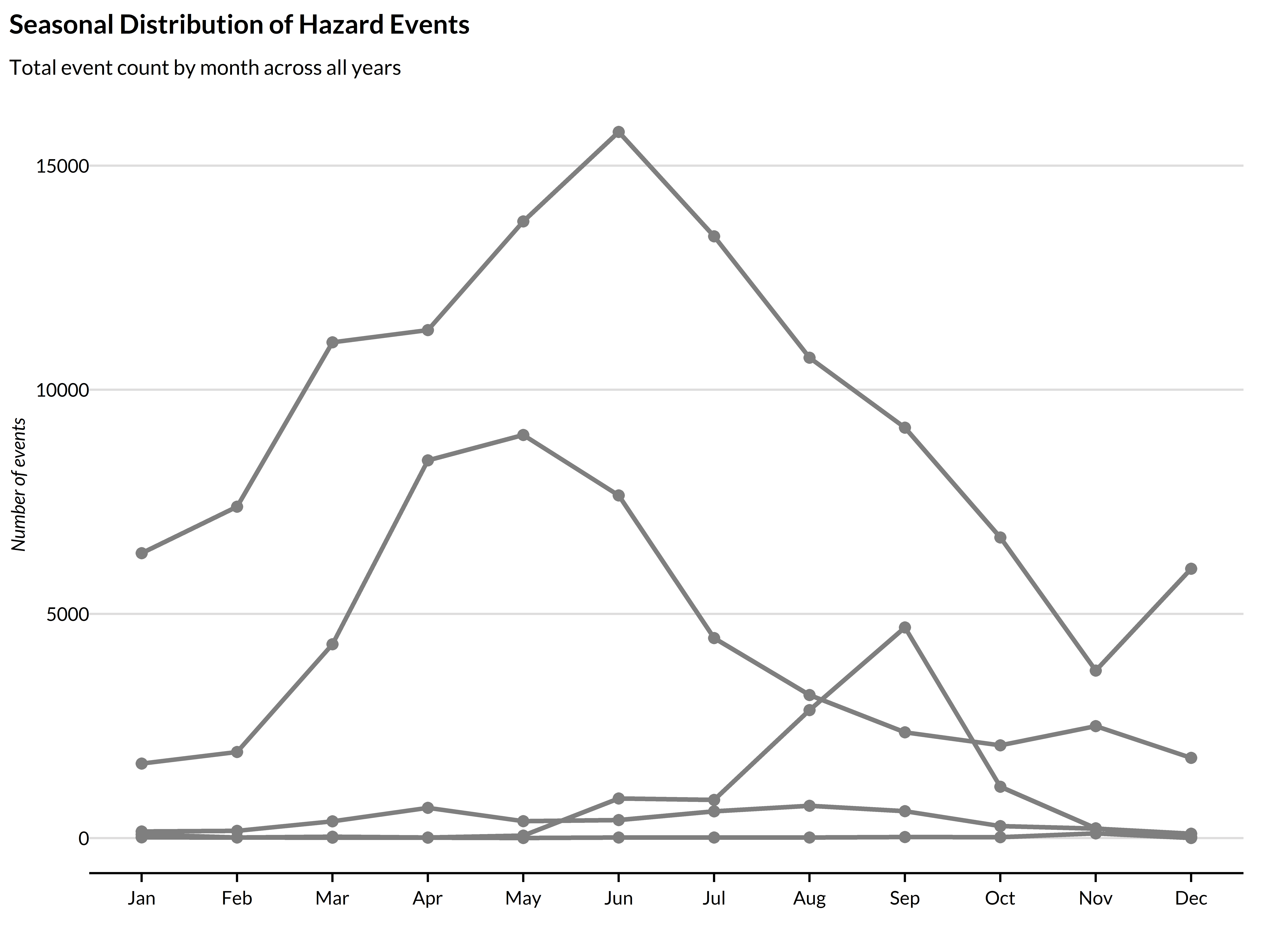

plot of chunk seasonal-patterns

Counties with highest fatalities

high_fatality_counties <- sheldus |>
  summarize(
    .by = c(GEOID, state_name, county_name),
    total_fatalities = sum(fatalities, na.rm = TRUE)) |>
  slice_max(total_fatalities, n = 15)

high_fatality_counties |>
  mutate(
    county_label = str_c(county_name, ", ", state_name),
    county_label = fct_reorder(county_label, total_fatalities)) |>
  ggplot(aes(y = county_label, x = total_fatalities)) +
  geom_col() +
  labs(
    title = "Counties with Highest Hazard-Related Fatalities",
    x = "Total fatalities",
    y = "")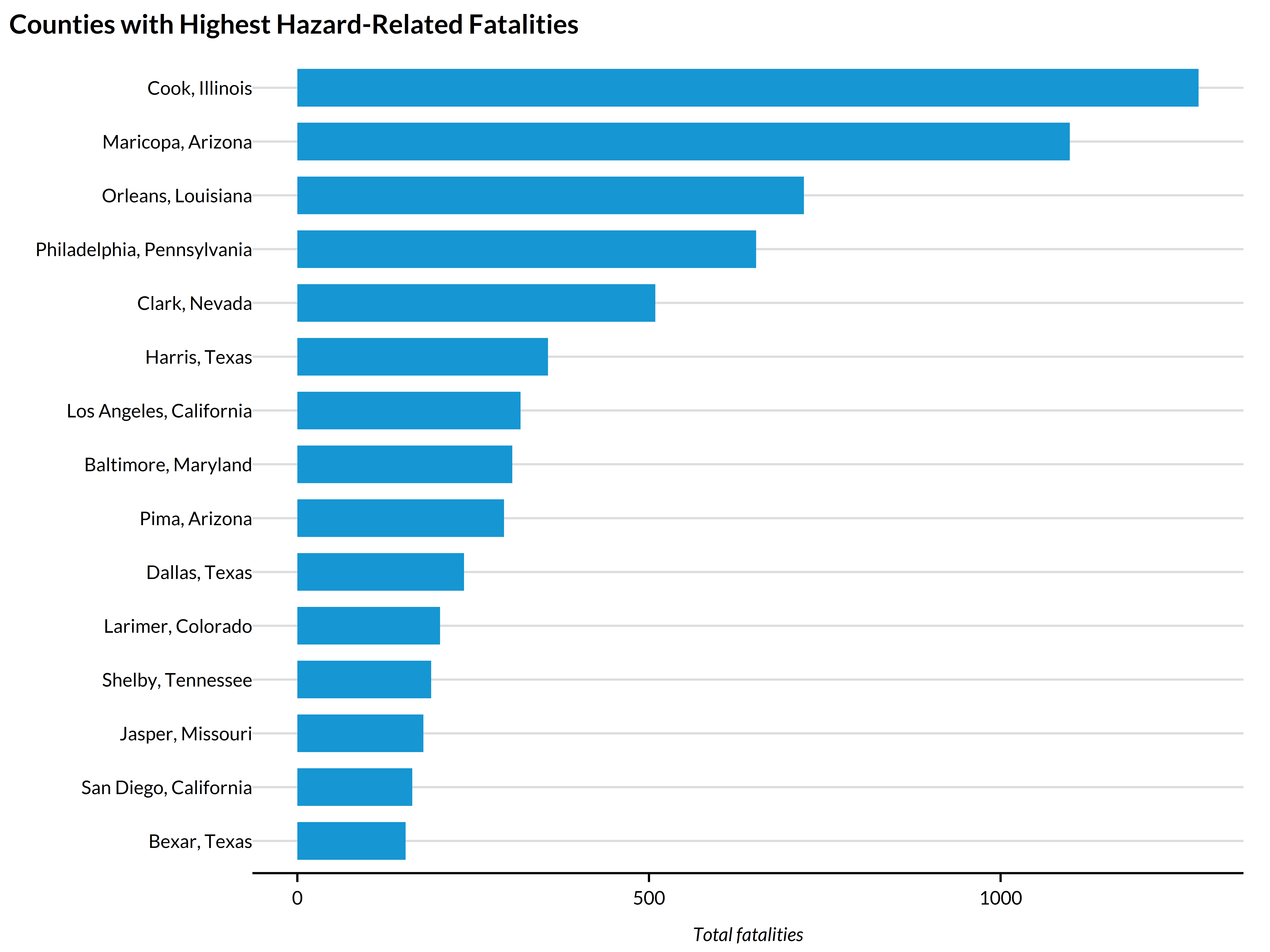

plot of chunk fatalities

Linking with census data

The county-level structure makes it straightforward to join with demographic data.

county_demographics <- tidycensus::get_acs(
  geography = "county",
  variables = c(
    median_income = "B19013_001",
    total_pop = "B01003_001"),
  year = 2022,
  output = "wide")

county_hazard_summary <- sheldus |>
  filter(year >= 2018) |>
  summarize(
    .by = GEOID,
    total_damage = sum(damage_property, na.rm = TRUE),
    total_events = sum(records, na.rm = TRUE)) |>
  left_join(county_demographics, by = "GEOID") |>
  mutate(damage_per_capita = total_damage / total_popE)