USA Structures Data
get_structures.RmdOverview
The get_structures() function retrieves building
footprint data from the USA Structures dataset and summarizes structure
counts by type at the tract or county level. This is useful for
estimating the number and types of buildings within areas affected by
natural hazards.
Data source
Data are sourced from the USA Structures dataset maintained by the Department of Homeland Security. The dataset contains building footprints derived from high-resolution imagery for structures across the United States.
See https://geoplatform.gov/metadata/9d4a3ae3-8637-4707-92a7-b7d67b769a6b for more information.
Loading the data
library(climateapi)
library(tidyverse)
library(sf)
library(urbnthemes)

set_urbn_defaults(style = "print")
The function requires a boundaries argument specifying
the geographic area of interest. This must be a spatial polygon object
with a defined coordinate reference system.
# Example: Get structures in Washington, DC
dc_boundary <- tigris::states(cb = TRUE) |>
  filter(STUSPS == "DC")

dc_structures <- get_structures(
  boundaries = dc_boundary,
  geography = "tract")
#> Reading layer `DC_Structures' from data source
#> `C:\Users\WCurranGroome\Box\METRO Climate and Communities Practice Area\github-repository\built-environment\housing-units\usa-structures\raw\DC\DC_Structures.gdb'
#> using driver `OpenFileGDB'
#> Simple feature collection with 64701 features and 33 fields
#> Geometry type: MULTIPOLYGON
#> Dimension: XY
#> Bounding box: xmin: -77.11509 ymin: 38.79307 xmax: -76.90971 ymax: 38.99554
#> Geodetic CRS: WGS 84Function parameters
-
boundaries: A POLYGON or MULTIPOLYGON sf object, or ansf::st_bbox()-style bounding box. Must have a defined CRS. -
geography: The desired output geography. One of"tract"or"county". -
keep_structures: IfTRUE, returns both the summarized counts and the raw point-level structure data.
Data structure
Each row represents a unique combination of geographic unit (tract or county) and structure type.
glimpse(dc_structures)
#> Rows: 1,951
#> Columns: 4
#> $ GEOID             <chr> "11001000101", "11001000101", "11001000101", "11001000101", "11001000101", "11001000101", "11001000102", "11001000102", "11001000102", "11001…
#> $ primary_occupancy <chr> "Single Family Dwelling", "Multi - Family Dwelling", "Religious", "Retail Trade", "General Services", "Temporary Lodging", "Single Family Dwe…
#> $ occupancy_class   <chr> "Residential", "Residential", "Assembly", "Commercial", "Government", "Residential", "Residential", "Residential", "Commercial", "Commercial"…
#> $ count             <int> 63, 24, 5, 4, 1, 1, 384, 48, 42, 21, 19, 15, 13, 10, 8, 5, 5, 4, 2, 1, 1, 53, 8, 8, 1, 1, 1, 310, 60, 42, 23, 12, 9, 8, 7, 3, 3, 3, 3, 2, 2, …
Key variables include:
-
GEOID: Census tract (11-digit) or county (5-digit) FIPS code -
primary_occupancy: The primary use of the structure (e.g., “Residential”, “Commercial”) -
occupancy_class: Broader classification of occupancy type -
count: Number of structures of this type in the geographic unit
Occupancy types
dc_structures |>
  distinct(occupancy_class, primary_occupancy) |>
  arrange(occupancy_class, primary_occupancy)
#> # A tibble: 27 × 2
#>    occupancy_class primary_occupancy
#>    <chr>           <chr>
#>  1 Assembly        Indoor Arena
#>  2 Assembly        Religious
#>  3 Commercial      Entertainment and Recreation
#>  4 Commercial      Hospital
#>  5 Commercial      Medical Office/Clinic
#>  6 Commercial      Parking
#>  7 Commercial      Personal and Repair Services
#>  8 Commercial      Professional/Technical Services
#>  9 Commercial      Retail Trade
#> 10 Commercial      Theaters
#> # ℹ 17 more rows
Example analyses
Structure composition by tract
dc_summary <- dc_structures |>
  summarize(
    .by = GEOID,
    total_structures = sum(count, na.rm = TRUE),
    residential = sum(count[occupancy_class == "Residential"], na.rm = TRUE),
    commercial = sum(count[occupancy_class == "Commercial"], na.rm = TRUE)) |>
  mutate(
    residential_share = residential / total_structures)

dc_summary |>
  ggplot(aes(x = total_structures, y = residential_share)) +
  geom_point(alpha = 0.7) +
  scale_y_continuous(labels = scales::percent) +
  labs(
    title = "Residential Share vs. Total Structures by Tract",
    subtitle = "Washington, DC census tracts",
    x = "Total structures",
    y = "Share residential")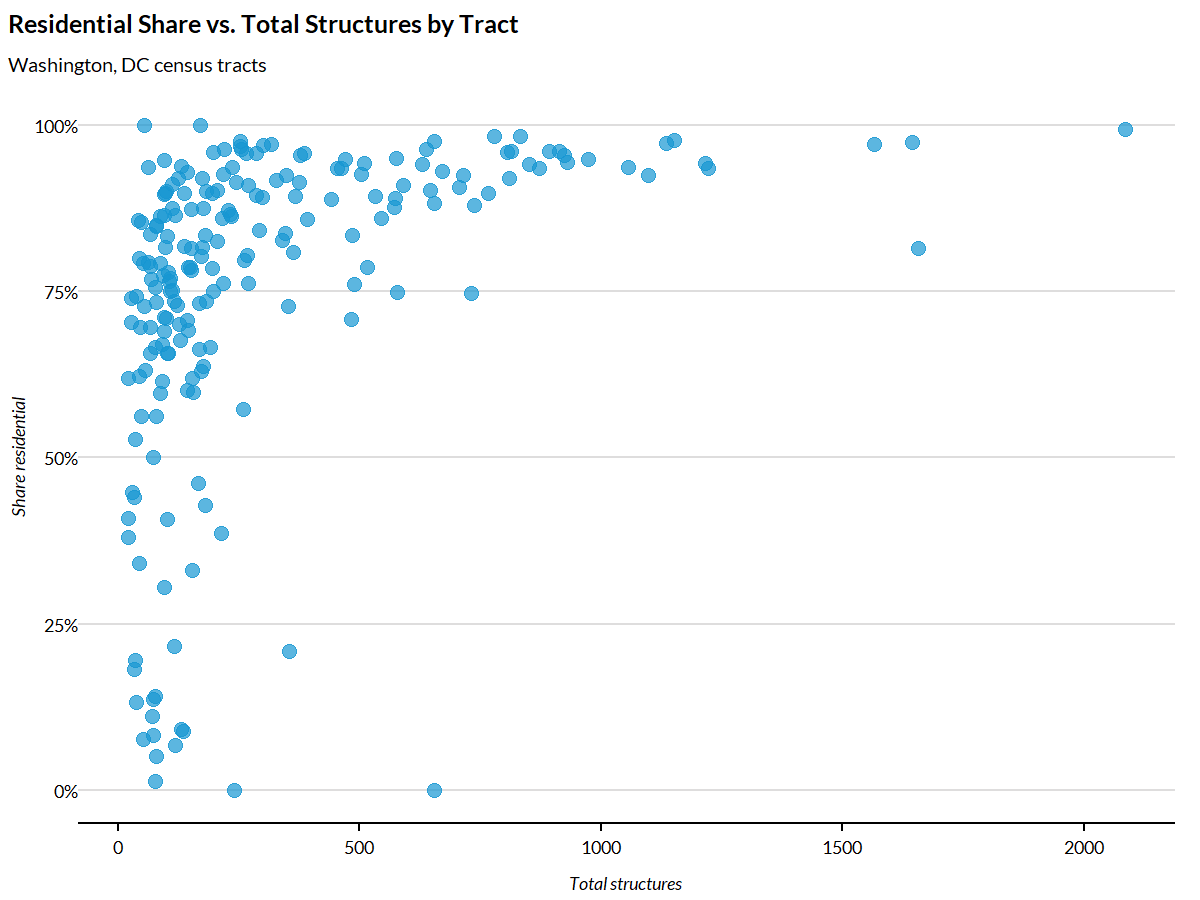
Mapping structure density
dc_tracts <- tigris::tracts(state = "DC", cb = TRUE, year = 2023, progress_bar = FALSE) |>
  st_transform(5070)

dc_tract_totals <- dc_structures |>
  summarize(
    .by = GEOID,
    total_structures = sum(count, na.rm = TRUE))

dc_map <- dc_tracts |>
  left_join(dc_tract_totals, by = "GEOID")

ggplot(dc_map) +
  geom_sf(aes(fill = total_structures), color = "white", linewidth = 0.2) +
  scale_fill_gradientn(
    colors = c(palette_urbn_cyan[1], palette_urbn_cyan[4], palette_urbn_cyan[7]),
    labels = scales::comma) +
  labs(
    title = "Structure Count by Census Tract",
    subtitle = "Washington, DC",
    fill = "Structures") +
  theme_urbn_map()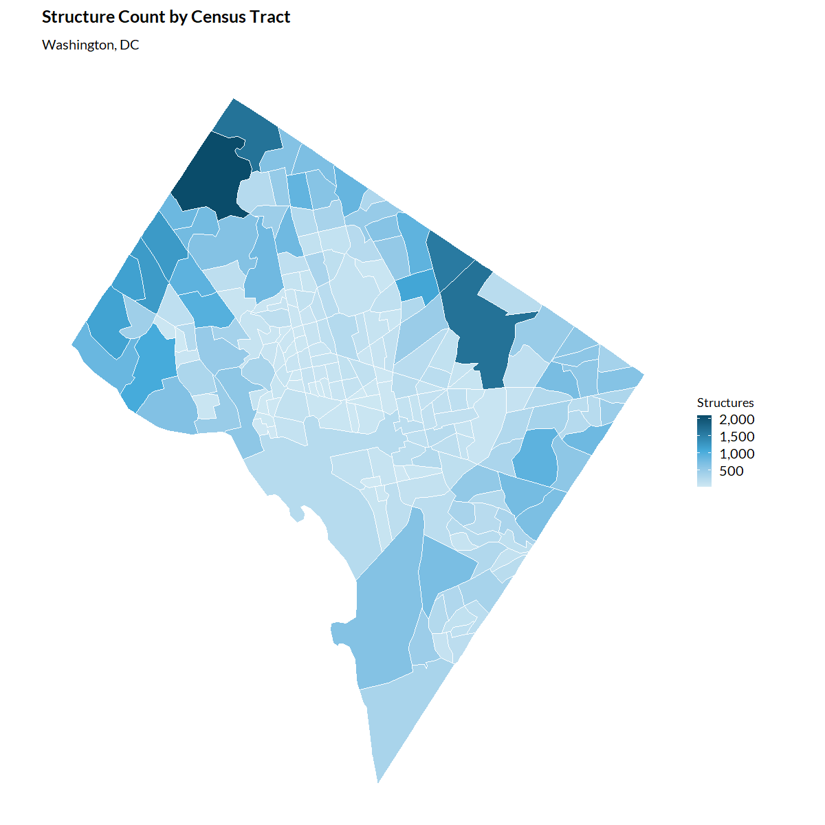
Analyzing structures in a disaster area
A common use case is estimating structures within a hazard-affected area. This example shows how to combine structure data with wildfire burn zones.
# Get a specific wildfire's burn zone
burn_zones <- get_wildfire_burn_zones()

camp_fire <- burn_zones |>
  filter(str_detect(wildfire_name, "CAMP"))

# Get structures within the burn zone
camp_fire_structures <- get_structures(

  boundaries = camp_fire,
  geography = "tract",
  keep_structures = TRUE)

# Summarized counts
camp_fire_structures$structures_summarized |>
  summarize(
    .by = occupancy_class,
    total = sum(count, na.rm = TRUE)) |>
  arrange(desc(total))
Working with raw structure data
Setting keep_structures = TRUE returns both the
summarized data and the raw point-level structure data.
dc_full <- get_structures(
  boundaries = dc_boundary,
  geography = "county",
  keep_structures = TRUE)

# Access the raw point data
raw_structures <- dc_full$structures_raw

# Access the summarized data
summary_structures <- dc_full$structures_summarized

# Map individual structures
ggplot() +
  geom_sf(data = dc_boundary, fill = "grey95") +
  geom_sf(
    data = raw_structures |> filter(primary_occupancy == "Commercial"),
    size = 0.1,
    alpha = 0.5) +
  labs(title = "Commercial Structures in Washington, DC") +
  theme_urbn_map()
County-level analysis
For larger areas, county-level aggregation provides a useful summary.
# Get structures for multiple states
southeast_boundary <- tigris::states(cb = TRUE) |>
  filter(STUSPS %in% c("FL", "GA", "AL", "SC"))

southeast_structures <- get_structures(
  boundaries = southeast_boundary,
  geography = "county")

# Summarize by county
county_totals <- southeast_structures |>
  summarize(
    .by = GEOID,
    total_structures = sum(count, na.rm = TRUE))
Performance considerations
The raw building footprint data files are large. Processing can be slow, especially for multi-state analyses. Consider:
- Starting with a small geographic area to test your workflow
- Using county-level aggregation when tract-level detail is not required
- Caching results for repeated analyses
See also
-
get_wildfire_burn_zones(): Wildfire burn zone disasters for use as boundaries -
get_current_fire_perimeters(): Active wildfire perimeters for use as boundaries -
get_fema_disaster_declarations(): FEMA disaster declarations