3 Synthetic Data

Published

April 23, 2026

Abstract

Synthetic data is a dataset designed to imitate a confidential dataset while limiting information about individual records in the confidential dataset. This chapter introduces the process of generating synthetic data.

Overview

In this chapter, you will learn about:

Synthetic data concepts.
Modeling and sampling design choices for synthetic data.
Best practices and considerations for making synthetic data design decisions.

3.1 Foundations

Before covering synthetic data, we start with a few foundational concepts.

3.1.1 Probability distributions

Definition: Joint Probabilities

Joint probabilities describe the probability of the co-occurrence of two or more events.

For example, what is the probability that a student attended College 1 and is a STEM major?

Definition: Conditional Probabilities

Conditional probabilities describe the probability of one event occurring given information about others.

For example, what is the probability that a student is a STEM major, given they attended College 1?

Class Activity 1

Institution	STEM	Non-STEM	Total
College 1	0.10	0.15	0.25
College 2	0.50	0.25	0.75
Total	0.60	0.40	1.00

Compute the two probabilities below:

If you do not have access to a computer, describe how you would carry out these calculations. For example, indicate which equation you would use and what values you would input.

What is the probability that a student attended College 1 and is a STEM major?
What is the probability that a student is a STEM major, given they attended College 1?

Compute the two probabilities below:

If you do not have access to a computer, describe how you would carry out these calculations. For example, indicate which equation you would use and what values you would input.

What is the probability that a student attended College 1 and is a STEM major? 0.10 or 10%
What is the probability that a student is a STEM major, given they attended College 1? 0.10 / 0.25 = 0.40 or 40%

3.1.2 Models

A model is a simplified mathematical representation of a system; for our purposes, we’re concerned with models that aim to replicate key relationships between variables in tabular data.

Suppose we have data about the speed of a car when the brake is hit and the distance it takes for the car to stop.

speed	dist
4	2
4	10
7	4
7	22
8	16
9	10

We can develop a simple model of the stopping distance using linear regression. This model isn’t perfect, but it does a reasonable job of approximating the real world with just two numbers.

(Intercept)       speed 
 -17.579095    3.932409

We can use these two numbers to predict the stopping distance of cars for any given speed.

speed	dist	dist_predicted
4	2	-1.849460
4	10	-1.849460
7	4	9.947766
7	22	9.947766
8	16	13.880175
9	10	17.812584

This model is a discriminative model that estimates the conditional mean of the stopping distance given the speed (\(E[Y|X]\) or \(P(Y|X)\)). Social scientists working on prediction problems, policy evaluations, or traditional explanatory and/or causal modeling are primarily concerned with discriminative models.

To generate synthetic data, we need generative modeling, which models the joint distribution of both \(Y\) and \(X\), i.e. \(P(Y, X)\). Recall that \(P(Y, X) = P(Y \mid X) P(X)\).

Most black-box models require data generating assumptions to convert \(E[Y \mid X]\) into \(P(Y \mid X)\).
Some predictive models, like linear models, imply specific generative relationships for \(P(Y \mid X)\). For example, linear regression implies \(P(Y \mid X)\) is normally distributed with the mean equal to the conditional mean from the discriminative model and the standard deviation equal to the residual standard error. This allows us to create plausible new observations that capture the variability in the original data.

3.1.3 Synthetic Data <-> Imputation Connection

Synthetic data has much in common with missing data problems like imputation:

Multiple imputation was originally developed to address non-response problems in surveys (Donald B. Rubin 1977).
Statisticians created new observations or values to replace the missing data by developing a generative model based on other available respondent information.
This process of replacing missing data with substituted values is called imputation.

Running Example: Imagine you are running a conference with 80 attendees. You are collecting names and ages of all your attendees. Unfortunately, when the conference is over, you realize that only about half of the attendees listed their ages. One common imputation technique is to just replace the missing values with the mean age of those in the data.

Figure 3.2 shows the distribution of the 40 age observations that are not missing.

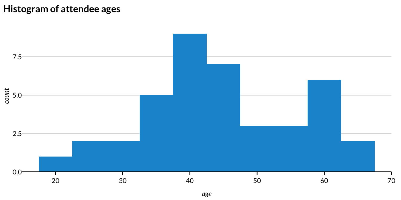
Figure 3.2: The distribution excluding missing values

Figure 3.3 shows the histogram using simple mean imputation. The results aren’t very good!

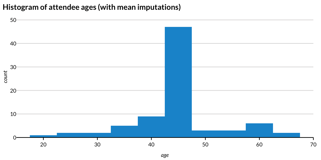
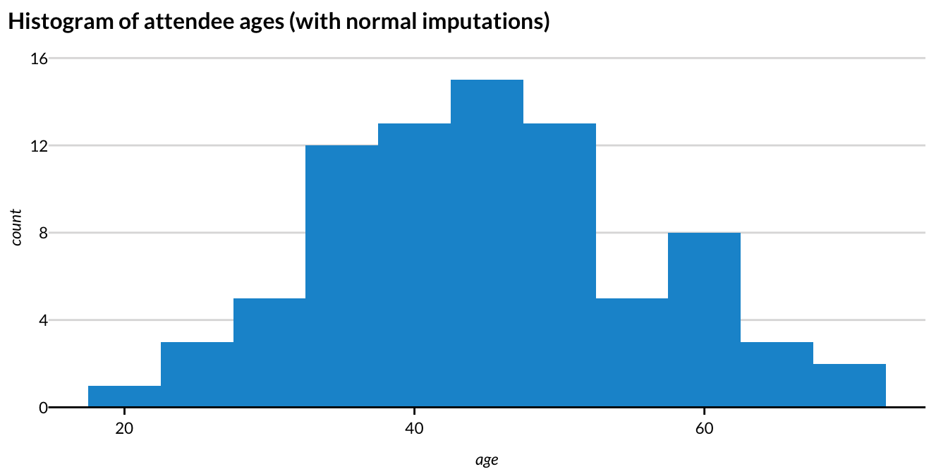
Figure 3.3: The distribution with simple mean imputation

Figure 3.4 shows the histogram using a normal distribution to impute missing values.

Figure 3.4: The distribution with imputations from a distribution

Using the mean to impute the missing ages removes useful variation and conceals information from the “tails” of the distribution.
We then draw from a normal distribution that used the sample mean and sample standard deviation from the non-missing values. The resulting distribution looked much more plausible.
When creating synthetic data, this process is repeated for an entire variable, or set of variables.
In a sense, the entire column is treated as missing!

3.1.4 Connections to other sampling techniques

Many problems in quantitative social science methods deal with missing data:

In statistical modeling, we may model the probability of missingness.
- e.g., “Which students are more or less likely to complete a course evaluation?”
In survey statistics, we may characterize potential respondents who did not complete a survey.
- e.g., “Which people are more or less likely to complete the American Community Survey?”
In causal inference, we may model what happened if a unit received a different treatment.
- e.g., “What might happen if a college graduate didn’t finish their degree?”

Note: Connections between synthetic and missing data

Synthetic data problems are examples of a special class of missing data problem with two key properties.

All complete data, i.e., confidential data, are deemed missing.*
We are intentionally designing the missingness mechanism.

3.2 What is synthetic data?

Definition: Synthetic Data

Synthetic data is a dataset designed to imitate a confidential dataset while limiting information about individual records in the confidential dataset.

Definition: Confidential Data

Confidential data is a dataset that contains personal or sensitive information that is, in general, not publicly accessible without specific provisions (for example, applying for restricted use permission).

Definition: Gold standard dataset

Gold standard dataset (GSDS) is a dataset produced from the confidential data that has the same form, structure, data representations, and tabular properties as the resulting synthetic data. Synthetic data algorithms use a GSDS as input to produce a synthetic dataset with the same form as the GSDS.

IMPORTANT: Data pre-processing

Throughout these materials, we assume that the confidential data represents the end result of any preprocessing steps needed to prepare the synthesis inputs, such as recoding variables, correcting structural errors, etc. In practice, confidential data and GSDSs may differ.

Key Points About Synthetic Datasets:

Synthetic datasets mimic the statistical properties of confidential datasets that are typically inaccessible to most users.
They are usually generated by randomly sampling records from trained generative models.
The goal is to preserve data utility by closely replicating the distribution and relationships in the original data, while minimizing disclosure risks.
Synthetic values limit the ability to make accurate or confident inferences about confidential data subjects, reducing the risk of re-identification.
Synthetic data can be used as a “training dataset” to develop and test code, which is later run on confidential data via a secure validation server.

3.2.1 Misconceptions of Synthetic Data

Note: What can we do with synthetic data?

Synthetic data enables easier data sharing for exploratory data analysis, data pipeline integration, and prototype program evaluations.

Example synthetic data use cases:

Expanding access to descriptive statistics for policymakers.
Providing policy researchers another means to access the GSDS to develop program evaluation analyses.
Helping data providers understand how to design systems that integrate with the target GSDS.

WARNING: No silver bullet

Synthetic data can be generated in many different ways, but synthetic data does not eliminate all possible disclosure risk harms.

Synthetic data, like any other PET, cannot ever eliminate all possible privacy risks.
Synthetic data, like any other PET, requires contextually specific evaluations of data utility and disclosure risks.
No universal metric fits all; risk is context-specific and multidimensional.
Code and documentation must be reviewed, as transparency can increase disclosure risk.

The mere presence of synthetic data does not automatically ensure adequate disclosure protection. Simply put, synthetic data can be generated in many different ways, but synthetic data does not eliminate all possible disclosure risk harms. The level of disclosure risk protection afforded by synthetic data is a function of how the synthetic data is generated, not the mere fact that the resulting dataset is named a “synthetic” dataset. For example, consider a “synthetic” dataset where 99% of records are identical to the confidential dataset. This dataset may be labeled “synthetic,” but it still poses significant disclosure risks.

Disclosure risk metrics measure the extent to which a statistical output may reveal information about individual records in confidential data. A key consideration when selecting metrics for disclosure risk evaluation is understanding that all non-trivial statistical outputs carry some level of disclosure risk. The only way to guarantee zero disclosure risk is to not release any data or information from the confidential data.

In other words, disclosure risk is contextually specific and multidimensional, by necessity, there are no standardized “one-size-fits-all” metrics or evaluation techniques for disclosure risk measurement. For example, data curators may care about the ability to infer the presence or absence of particular records more than others. Similarly, data curators may wish to assess the influence of certain data curator’s contributions on a resulting synthetic dataset. By construction, no synthetic data solution can ever address every dimension of this problem simultaneously and with certainty.

Additionally, the code and documentation used to generate synthetic data should be reviewed independently for disclosure risks. In general, greater methodological transparency increases disclosure risk for all data products. Therefore, all code, documentation, and other supplemental materials related to data product publication should be reviewed for potential disclosure. For example, information about data collection frames and response rates can be used to reverse engineer sample demographics and should be published with discretion. Similarly, code details related to pseudo-random number generation should be excluded to prevent replication of randomness and potential re-identification.

WARNING: Data are data

Synthetic data are not fake data, and confidential data are not real data.

All data are made, not found; synthetic data refers to only one part of the data-making process.
Synthetic data enables transparent communication about how data are made, including but not limited to the synthesis process.

All data are made, not found. Government and private sector entities undertake important, rigorous work to transform raw data inputs into high-quality and easily usable datasets well before ever considering synthesis. As a result, synthetic data refers to only one part of the data-making process.

The word “synthetic” can evoke negative connotations about data appearing inauthentic or deceptive. Such connotations often deter data curators from adopting synthetic data due to anxieties about institutional or reputational harms from releasing “fake” data products. Although concerns about data quality and responsible data usage are important, these concerns apply to any data product, synthetic or not. Modifications to raw data (i.e., the collected data that are unaltered), such as input error correction, imputations of missing values, or record linkages, result in statistical decisions by a user that affect the analysis. Alternatively, synthesis should be viewed as another part of the data-making process, where greater transparency about data-production processes can enable more responsible use.

WARNING: Synthetic data are different than confidential data

Data users should not assume to use the synthetic data the same way they would confidential data.

Don’t blindly replace confidential data with synthetic data.
Educate users with clear disclaimers and guidance.
Synthetic data accuracy depends on design and purpose.
Use utility metrics aligned with intended use.
Validate when applying data beyond original scope.
Consider user interaction, metrics, and result sharing.
Provide full documentation to support evaluation and adoption.

New users of synthetic data may be tempted to directly substitute confidential data for synthetic data, but making this substitution without additional considerations could be dangerous in the wrong setting. User education is the most effective tool to enable responsible use and prevent potential misuse. Most importantly, responsible user education starts with explicit disclaimers about how synthetic data was generated and what the synthetic data should and should not be used for in downstream applications. More comprehensive user education can take many forms, including reporting on synthetic data evaluations, trainings, and other learning resources.

Because synthetic data are designed to mimic confidential data, potential users may mistakenly assume they can answer the same questions with same amount of accuracy or certainty. However, the synthetic data usefulness depends on how they are constructed, the intended analytical purpose, and other factors considered during the synthetic data generation process.

Like disclosure risk metrics, utility metrics assess how well synthetic data support downstream analysis. These metrics should be based on the intended use cases, which may not cover all possible applications.

When users wish to apply synthetic data beyond its original purpose, validation processes can help. These allow users to compare results from synthetic data to those that might be produced using confidential data. When considering a validation process, some key design questions include but are not limited to:

User interaction: Will users submit manual requests or use automated systems like validation query interfaces?
Metrics provided: Will users receive exact statistics or privacy-preserving outputs using PETs?
Use of results: Will validation results be publicly released, or selectively shared due to disclosure risks?

Another consideration is ensuring complete and accurate documentation (e.g., code, model specifications, and data processing decisions). These are essential for evaluating utility and supporting broader adoption.

3.3 Overall Synthesis Workflow

Effective synthetic data deployment involves multiple steps, outlined in Figure 3.5. Note that while these steps occur in sequential order, feedback from one step may require revisiting a previous step. As a result, synthetic data generation and evaluation is an iterative, collaborative process among all stakeholders.

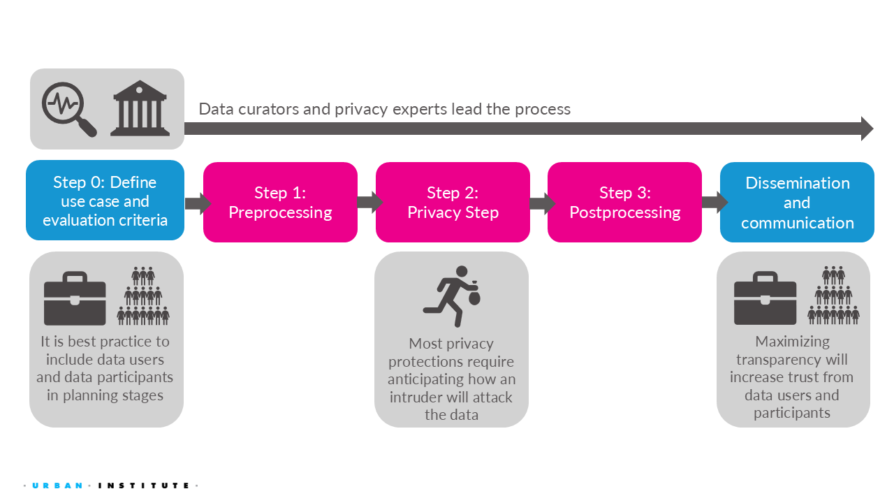
Flowchart of a data privacy process led by curators and experts. Steps: 0) Define use case and thresholds → 1) Preprocessing → 2) Privacy Step → 3) Postprocessing → Dissemination and communication. Notes: include data users early, anticipate intruder attacks, and maximize transparency for trust. — Figure 3.5: All of the privacy stakeholders discussed previously have a role in aspects of the synthesis process.

3.3.1 Define Use Cases and Goals (Step 0).

Data curators work with data users and subjects to define use cases for synthetic data.

Work with data users and stakeholders to identify supported use cases and utility goals.
Design utility benchmarks using both quantitative and qualitative methods.
Work with data providers and disclosure review decision makers to identify disclosure risk evaluation strategy and decision criteria. Decisions should be informed by laws, threat models, and available external data sources.
Design privacy benchmarks using both quantitative and qualitative methods. Review code and documentation to manage transparency-related risks.

This critical step ensures that synthetic data meets the needs of prospective data users, which may vary significantly. Creating clear data utility goals ensures generating synthetic data serves an explicit data user purpose; otherwise, data curators risk releasing more data for more data’s sake alone.

Data user needs typically vary widely. Some data users may only need to compute summary statistics on a few key variables, such as demographic information. Other users may need more granular information, such as record-level microdata for subpopulations of interest. As part of this process, data curators can identify data use requirements, or goals for the success of a particular synthetic data task. For example, suppose program evaluators currently use restricted access data to evaluate a suite of programs. Data curators may want to produce statistics that differ by a relative error of no more than 10 percent from those based on the confidential data for said programs.

A similar process is necessary for identifying potential disclosure risks involving data users, data subjects, and legal counsel. Several factors must be considered, including relevant laws and regulations, how legal counsel interprets those laws, and potential threat models that impact the data subjects. Assessing threat models may involve conducting a landscape scan of external resources, such as other data products derived from the confidential data or similar datasets available outside the original source that could be used to infer sensitive information from the synthetic data. Privacy experts then partner with these stakeholders to design quantitative and qualitative benchmarks based on these threat models. All these factors should inform the design and evaluation of disclosure risk metrics to ensure robust privacy protection.

3.3.2 Preprocess and Create a Gold Standard Data (Step 1).

Data curators and privacy experts work together to preprocess the data.

The GSDS is designed to match the structure of the synthetic dataset.
GSDS design varies by use case (e.g., student-level vs. course-level data).
Synthetic data always aims to imitate a specific GSDS, not the original raw data.

The goal of this stage is to design and create a GSDS, or a confidential dataset that has the exact same form as the resulting synthetic dataset. Synthetic data always aims to imitate one specific GSDS, but there are many possible ways to design and produce GSDSs. For example, some education researchers may be interested in student-level synthetic data (one record per student), whereas others may be interested in course-level synthetic data (one record per instance of a particular course).

In the next two steps, data privacy experts generate and evaluate our synthetic data.

3.3.3 Privacy Step - Synthesis and Testing (Step 2).

As mentioned before, there are many ways to generate the synthetic data file, such as using a statistical and/or algorithmic modeling techniques to generate synthetic data based on the GSDS.

3.3.4 Post-process – Evaluating (Step 3).

Once the synthetic file is generated, it should be evaluated using a range of metrics that reflect the privacy and utility goals established during Step 0.

Steps 2 and 3 are often performed iteratively; one might evaluate multiple synthetic data configurations or try new synthetic data configurations motivated by evaluation results.

3.3.5 Dissemination and Communication (Step 4).

Synthetic data are disseminated to potential data users.

Users must understand how data were generated, evaluated, and intended to be used.
Implementation decisions affect how much information about the synthesis process can be safely communicated.
Clearly communicate appropriate use cases and limitations (e.g., suitable for contingency tables, not complex modeling).

Here it is critical to make sure the data users are well-informed about how the synthetic data were generated, how the synthetic data were evaluated, and how the synthetic data should be used in practice. For example, if a synthetic dataset is sufficiently accurate for producing and using two-way contingency tables in exploratory analyses but not for complex nonparametric modeling, data users need to know this information to responsibly use their synthetic data. At the same time, details about how the synthetic data were created can create risks because an attacker could use this information to reverse-engineer confidential information.

Note: Increase trust in the data ecosystem

Throughout all these steps, the data curator and privacy experts should be transparent by ensuring proper communication of the process with data users and data subjects.

Good example of transparency: The data steward provides examples of relationships between categorical variables and the degree to which they are preserved or not preserved in the synthetic data.
Bad example of transparency: The data steward shares the exact code and pseudo-random-number generating seed used to produce synthetic data.

3.4 Major Design Decisions for Synthetic Data

The following decisions affect the macroscopic approach to synthesizing data:

Partial vs. fully synthetic data: are any relationships to the confidential data units preserved?
Plausible values: what forms of validity will be preserved by the synthesis process?
Dimensions: what size and shape will the resulting synthetic dataset(s) take?

3.4.1 Partially vs. Fully synthetic

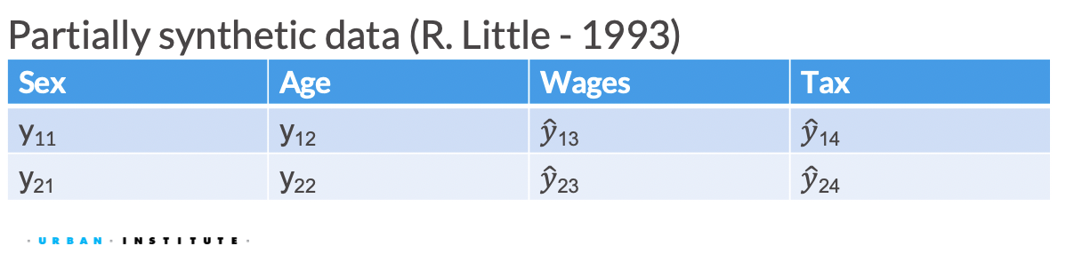
Definition: Partially Synthetic

Partially synthetic data only synthesizes some observations or variables in the released data (generally those most sensitive to disclosure). In partially synthetic data, there remains a one-to-one mapping between confidential records and synthetic records.

In Figure 3.6, we see an example of what a partially synthesized version of the above confidential data could look like.

Definition: Fully Synthetic

Fully synthetic data synthesizes all values in the dataset. Fully synthetic data no longer directly map onto the confidential records.

In Figure 3.7, we see an example of what a fully synthesized version of the confidential looks like.

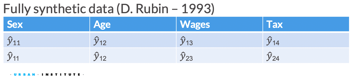
More details about generating fully synthetic data according to the original proposal in D. B. Rubin (1993) can be found in J. Drechsler (2011), Raghunathan, Reiter, and Rubin (2003), and J. P. Reiter and Raghunathan (2007).

Class Activity 2

This conceptual activity will explore the difference between partial and fully synthetic data.

Consider the penguins data.

species	bill_length_mm	sex

Chinstrap	51.3	male
Gentoo	44.0	female
Chinstrap	51.4	male
Chinstrap	45.4	female
Adelie	36.2	female

Let’s say that researchers decide that the sex of the penguins in the data are not confidential, but the species and bill length are. So, they develop regression models that synthesize species conditional on sex and synthesize bill_length conditional on species and sex. They then use those models to synthesize species and bill lengths for each row in the data.

What specific Statistical Disclosure Control method are these researchers using?

They are using partially synthetic data.

Class Activity 3

This conceptual exercise explores the trade offs between partially and fully synthetic data.

Shown here are the first seven rows of a dataset about the prices and attributes of diamonds. Suppose you decide to synthesize the “price” variable, because that information is too sensitive for public release.

price	carat	cut	color	clarity
326	0.23	Ideal	E	SI2
326	0.21	Premium	E	SI1
327	0.23	Good	E	VS1
334	0.29	Premium	I	VS2
335	0.31	Good	J	SI2
336	0.24	Very Good	J	VVS2
336	0.24	Very Good	I	VVS1

After you synthesize the price variable, would the resulting dataset be considered partially or fully synthetic?

Partially synthetic

What are the trade-offs of a partially synthetic dataset compared to a fully synthetic dataset?

Describe in words how you would synthesize the “price” variable. Is the method you described parametric or non-parametric? Why?

What are the trade-offs of a partially synthetic dataset compared to a fully synthetic dataset?

Changing only some variables (partial synthesis) in general leads to higher utility in analysis since fewer variables are by definition unchanged (J. Drechsler and Reiter 2008).
Disclosure in fully synthetic data is challenging because all values are imputed, while partial synthesis has higher disclosure risk since confidential values remain in the dataset (J. Drechsler and Reiter 2008).
- Note that while the risk of disclosure for fully synthetic data can be very low, it is never zero.
Accurate and exhaustive specification of variable relationships and constraints in fully synthetic data are difficult and if done incorrectly can lead to bias (Jörg Drechsler, Bender, and Rässler 2008).
- If a variable is synthesized incorrectly early in a sequential synthesis, all variables synthesized on the basis of that variable will be affected.
Partially synthetic data may be publicly perceived as more reliable than fully synthetic data.

Describe in words how you would synthesize the “price” variable. Is the method you described parametric or non-parametric? Why?

3.4.2 Plausible Values

Synthetic data may need to conform to user’s structural assumptions for users to trust their results:

Randomization can lead to implausible values like negative test scores or fractional counts of people.
Randomization can also lead to implausible combinations of values like math grades for a student who didn’t take math.

High-quality synthetic data that support a range of useful analyses could contain implausible individual values and implausible combinations of values.

Some analyses may be affected on the frequency and severity of these deviations from structural assumptions. For example, one or two negative test scores may not affect analyses like over 50% negative test scores.
Many techniques exist to remedy these issues. These include using more complex distributions, resampling techniques, and enforcing univariate and multivariate constraints. However, these techniques often increase computation time and the potential for statistical bias.

3.4.3 Dimensions

Synthetic data need not have the same shape (specification of rows and columns) as the underlying confidential data:

Not all variables in a confidential dataset need to be synthesized or represented the same way:
- Some confidential variables can be omitted entirely.
- Some confidential variables can be modified prior to synthesis (for example, replacing exact income values with income ranges).
Similarly, fully synthetic data doesn’t need to have the same number of observations as the GSDS or confidential data.

Definition: Implicates

Implicates (also called replicates or synthetic datasets) are multiple versions of a synthetic dataset generated from the same confidential data. Each implicate represents an independent draw from the synthesis process.

Researchers can create any number of versions of a partially synthetic or fully synthetic dataset. Each version of the dataset is called an implicate. These can also be referred to as replicates or simply “synthetic datasets”
- For partially synthetic data, non-synthesized variables are the same across each version of the dataset.
Multiple implicates are useful for understanding the uncertainty added by imputation and are required for calculating valid standard errors.
More than one implicate can be released for public use; each new release, however, increases disclosure risk (but allows for more complete analysis and better inferences, provided users use the correct combining rules).
Implicates can also be analyzed internally to find which version(s) of the dataset provide the most utility in terms of data quality.

Class Activity 4

Multiple Implicates

What are the privacy implications for releasing multiple versions of a synthetic dataset (implicates)? Do these implications change for partially vs. fully synthetic data?

Releasing multiple implicates improves transparency and analytical value, but increases disclosure risk (violates “security through obscurity”).
It is more risky to release partially synthetic implicates, since non-synthesized records are the same across each dataset and there remains a 1-to-1 relationship between confidential and synthesized records.

3.5 Simple Synthesis Example

Suppose we wanted to generate synthetic data from a confidential dataset of three variables describing 4-year institution attendees, Institution, Major, and Age.

Here’s one possible strategy for generating synthetic data:

Fit a model for \(P(Inst)\).

\[ P(\text{Institution = College1}) = ?, \quad P(\text{Institution = College2}) = ?, \quad \text{etc.} \]

Sample new synthetic records for Institution from the model in step #1.

Confidential Data
Institution	Major	Age
College 1	English	22
College 2	Math	23
College 1	History	25
…	…	…

Synthetic Data
Institution	Major	Age
College 1
College 1
College 3
…

Fit a model for \(P(\text{Major | Institution})\).

\[ P(\text{Major = English | Institution = College1}) = ?, \dots \]

Append synthetic samples for Major by sampling from the model in step #3.

Confidential Data
Institution	Major	Age
College 1	English	22
College 2	Math	23
College 1	History	25
…	…	…

Synthetic Data
Institution	Major	Age
College 1	Math
College 1	English
College 3	Spanish
…	…

Fit a model for \(P(\text{Age | Institution, Major})\).

\[ P(\text{Age = 21 | Institution = College1, Major = English}) = ?, \dots \]

Append synthetic samples for Age by sampling from the model in step #5.

Confidential Data
Institution	Major	Age
College 1	English	22
College 2	Math	23
College 1	History	25
…	…	…

Synthetic Data
Institution	Major	Age
College 1	Math	21
College 1	English	22
College 3	Spanish	23
…	…	…

3.6 Implementation Decisions

IMPORTANT: Model choice matters

Synthetic data are only as good as the models and samplers used for generative modeling!

3.6.1 Generative Models

Definition: Generative Models

Generative models are models that describe the joint distribution of random variables. For example, \(P(X, Y)\) could describe an observable variable \(X\) and outcome variable \(Y\).

If we have an observed \(x\), we can use the model to generate random instances of \(y\) given \(x\).

Synthetic data generation relies on two steps:

Modeling: construct a generative model for the relationships between variables.
Sampling: sample new values from the generative model in Step 1.

3.6.2 Sampling

Synthesis is not prediction. Most predictive models focus on predicting the most likely outcome with a conditional mean or conditional probabilities. High-quality synthetic data requires sampling from distributions of plausible values.

Accordingly, model selection requires a plan for how to sample from the models.

Bayesian vs. Frequentist

Bayesian modeling can be used to create posterior predictive distributions, which are very useful for imputation and synthetic data generation.

Bayesian synthesis models

For all Bayesian synthesis models, the general approach to generating synthetic data lies in the use of the posterior predictive distribution. Essentially, we can think of synthetic data as predictions generated from the posterior distribution of the model parameters estimated on the confidential dataset.

Let \(\boldsymbol{Y}\) represent the confidential dataset containing \(n\) observations and \(p\) variables and \(\boldsymbol{\theta}\) represent the parameters of the selected Bayesian model for \(\boldsymbol{Y}\). Denote \(f(\boldsymbol{Y} \mid \boldsymbol{\theta})\) as the sampling model and \(\pi(\boldsymbol{\theta})\) as the prior choice for \(\boldsymbol{\theta}\). By Bayes’ theorem, the posterior distribution of \(\boldsymbol{\theta}\) can be estimated by \[\begin{equation} \pi(\boldsymbol{\theta} \mid \boldsymbol{Y}) \propto \pi(\boldsymbol{\theta}) f(\boldsymbol{Y} \mid \boldsymbol{\theta}). \label{eq:posterior} \end{equation}\]

Through Markov chain Monte Carlo (MCMC) techniques of posterior estimation, we can generate posterior draws of parameters \(\boldsymbol{\theta}\), denoted as \(\tilde{\boldsymbol{\theta}}\). We can then simulate predictions of \(\boldsymbol{Y}\) from the sampling model using the collection of posterior samples, \(\tilde{\boldsymbol{\theta}}\). A synthetic dataset, denoted as \(\tilde{\boldsymbol{Y}}\) sharing the same dimension as the confidential dataset \(\boldsymbol{Y}\), can contain synthesized values of a subset of variables, and therefore being partially synthetic and correspond to the same observations as in \({\boldsymbol{Y}}\); or of all variables, and therefore being fully synthetic (i.e., using the partial synthesis approach) and do not correspond to the same observations as in \({\boldsymbol{Y}}\).

When we need to generate multiple synthetic datasets, we first simulate \(m\) independent sets of posterior parameters, \(\tilde{\boldsymbol{\theta}} = \{\tilde{\boldsymbol{\theta}}^{(1)}, \cdots, \tilde{\boldsymbol{\theta}}^{(m)}\}\), from the posterior estimation process through MCMC. Next, each synthetic dataset, \(\tilde{\boldsymbol{Y}}^{(l)}\) (\(l \in 1, \cdots, m\)), is generated from the sampling model using the set of parameter draws \(\tilde{\boldsymbol{\theta}}^{(l)}\). We denote the resulting \(m\) sets of synthetic datasets as \(\tilde{\boldsymbol{Y}} = \{\tilde{\boldsymbol{Y}}^{(1)}, \cdots, \tilde{\boldsymbol{Y}}^{(m)}\}\).

Frequentist synthesis models

We can also generate synthetic data from other types of models that are not in a Bayesian framework. This usually requires an ad hoc assumption to create conditional distribution. We roughly group these methods as nonparametric (e.g., synthetic data generation based from an empirical distribution) or parametric (e.g., synthetic data generation based from a parametric distribution or generative model).

Similar to Bayesian synthesis models, when implementing a parametric approach, it becomes crucial to select a suitable model that accurately represents the confidential data to preserve as many of the underlying data relationships as possible. One straightforward parametric method for generating synthetic data is selecting an appropriate probability distribution. This approach involves making random draws from the chosen distribution based on the parameters or sufficient statistics from the confidential data. For instance, if the confidential data follows a Gaussian distribution, we can generate the synthetic data by drawing random samples from a Gaussian distribution, utilizing the sample mean and variance obtained from the confidential data.

More complex models may include using prediction models, such as regression, or conducting a sequential synthesis that estimates models for each predictor with previously synthesized variables used as predictors. The latter approach captures more of the multivariate relationships (or joint distributions) without being too computationally expensive, as compared to estimating a complicated joint distribution of all predictors to be synthesized. We can select the synthesis order based on the priority of the variables or the relationships between them. Typically, if the variable is synthesized earlier in the order, then the confidential information for that variable is better preserved in the synthetic data. Claire McKay Bowen, Liu, and Su (2021) propose a method that ranks variable importance by either practical or statistical utility and sequentially synthesizes the data accordingly.

3.6.3 Models

Definition: Parametric Data Synthesis

Parametric data synthesis is the process of data generation based on a parametric distribution or generative model.

Parametric models assume a finite number of parameters that capture the complexity of the data.
They are generally less flexible, but more interpretable than nonparametric models.
For example, regression to assign an age variable, sampling from a probability distribution, Bayesian models, or copula based models.

Definition: Nonparametric Data Synthesis

Nonparametric data synthesis is the process of data generation that is based on a limited number of assumptions about the underlying distribution or model.

Often, nonparametric methods use frequency proportions or marginal probabilities as weights for some type of sampling scheme.
They are generally more flexible, but less interpretable than parametric models.
For example, assigning gender based on underlying proportions, CART (Classification and Regression Trees) models, RNN models, etc.

For the nonparametric approach, the most basic method is using marginal tables and random sampling. For instance, we can categorize the data into groups or bins, calculate the proportion, and randomly sample synthetic values based on the proportion. This approach is simple and quick to implement, but does not properly capture the variability and relationships of continuous variables because the continuous values get discretized C. M. Bowen and Liu (2020).

A more complex nonparametric technique is a sequence of Classification and Regression Tree (CART) models Gordon et al. (1984). Jerome P. Reiter (2005) originally proposes to use a collection of nonparametric models to generate partially synthetic data. Essentially, CART iteratively divides the data using binary splits until reaching homogeneous nodes. If the target variable is categorical, CART employs classification trees to predict the outcome that constructs the tree by progressively partitioning the data into binary segments. For continuous variables, CART uses regression trees to determine the splitting value that separates the continuous values into partitions. A regression tree generates nodes with the lowest sum of squared errors, calculated as squared deviations from the mean.

3.6.4 Sequential Synthesis

Directly modeling joint distributions is difficult. One trick to get around this is to break the joint distribution into conditional distributions and model each variable using previously synthesized variables as predictors. This iterative process is called sequential synthesis or fully conditional specification.

The process described above may be easier to understand with the following table:

Step	Outcome	Modelled with	Predicted with

1	Sex	—	Random sampling with replacement
2	Age	Sex	Sampled Sex
3	Social Security Benefits	Sex, Age	Sampled Sex, Sampled Age
—	—	—	—

We can select the synthesis order based on the priority of the variables or the relationships between them.
The earlier in the order a variable is synthesized, the better the original information is preserved in the synthetic data usually.
Claire McKay Bowen, Liu, and Su (2021) proposed a method that ranks variable importance by either practical or statistical utility and sequentially synthesizes the data accordingly.

Typically when synthesizing data, modeling a joint distribution can be mathematically and computationally challenging. However, we can model joint probabilities using conditional probabilities.

Confidential data: a table \(X\) with \(n\) rows and \(m\) columns. For example, a dataset with \(n\) students and \(m\) descriptions of the student demographics (e.g., age, gender, county of residence, etc.).
Confidential data variables: \(X_j\) for \(j = 1, 2, 3 \dots, m\). For example, a column with \(n\) students’ ages.

\[ P(X) = P(X_1, \dots, X_m) = P(X_1) P(X_2 | X_1 ) \dots P(X_m | X_1, \dots, X_{m-1}) \]

This means we can break a large generative model into two parts:

A small generative model for some starting variables.
A sequence of conditional models for our remaining variables.

Class Activity 5

Sequential Synthesis (Conceptual)

You have a confidential dataset that contains information about dogs’ weight and their height. You decide to sequentially synthesize these two variables and write up your method below. Can you spot the mistake in writing up your method?

To create a synthetic record, first synthetic pet weight is assigned based on a random draw from a normal distribution with mean equal to the average of confidential weights, and standard deviation equal to the standard deviation of confidential weights. Then the confidential height is regressed on the synthetic weight. Using the resulting regression coefficients, a synthetic height variable is generated for each row in the data using just the synthetic weight values as an input.

To create a synthetic record, first synthetic pet weight is assigned based on a random draw from a normal distribution with mean equal to the average of confidential weights, and standard deviation equal to the standard deviation of confidential weights. Then the confidential height is regressed on the synthetic weight. Using the resulting regression coefficients, a synthetic height variable is generated for each row in the data using just the synthetic weight values as an input.*

height should be regressed on the confidential values for weight, rather than the synthetic values for weight

3.6.5 Simple Synthesis (Redux)

Let’s return to the example synthesis from above. Suppose we wanted to generate synthetic data from a confidential dataset of three variables describing 4-year institution attendees, Institution, Major, and Age.

Here’s a more detailed strategy for generating synthetic data:

Pick an order for sequentially synthesizing the joint distribution.

Here we will go from most complex to least complex categorical variables and then the numeric variable.

Fit a model for \(P(Inst)\). We can use the observed probabilities in the GSDS. We could add noise to these probabilities but we will not here.

\[ P(\text{Institution = College1}) = ?, \quad P(\text{Institution = College2}) = ?, \quad \text{etc.} \]

Sample new synthetic records for Institution from the model in step #2.

Confidential Data
Institution	Major	Age
College 1	English	22
College 2	Math	23
College 1	History	25
…	…	…

Synthetic Data
Institution	Major	Age
College 1
College 1
College 3
…

Fit a model for \(P(\text{Major | Institution})\). We will use a simple decision tree.

\[ P(\text{Major = English | Institution = College1}) = ?, \dots \]

Append synthetic samples for Major by sampling from the model in step #4.

Confidential Data
Institution	Major	Age
College 1	English	22
College 2	Math	23
College 1	History	25
…	…	…

Synthetic Data
Institution	Major	Age
College 1	Math
College 1	English
College 3	Spanish
…	…

Fit a model for \(P(\text{Age | Institution, Major})\). We will use a regression tree.

\[ P(\text{Age = 21 | Institution = College1, Major = English}) = ?, \dots \]

Append synthetic samples for Age by sampling from the model in step #6.

Confidential Data
Institution	Major	Age
College 1	English	22
College 2	Math	23
College 1	History	25
…	…	…

Synthetic Data
Institution	Major	Age
College 1	Math	21
College 1	English	22
College 3	Spanish	23
…	…	…

Class Activity 6

For synthetic data to work in practice, we have to make many design decisions, i.e., choices about how we want to process the confidential data to produce synthetic data.

What design decisions did we make (or would have to make) in the example above?

Starting variable(s): which variables will be part of the first generative model?
Variable order: in what order will be synthesize variables?
Model definitions: how will we compute \(P(X_2 \mid X_1)\) or \(P(X_3 \mid X_1, X_2)\)?
Sampler definitions: how will we draw new samples for \(X_1\), \(X_2 \mid X_1\), or \(X_3 \mid X_1, X_2\)?

3.7 Final Example

Class Activity 7: Sequential Synthesis (Computational)

For this exercise, we will use the starwars dataset from the dplyr package. We will practice sequentially synthesizing a binary variable (gender) and a numeric variable (height).

# run this to get the dataset we will work with
starwars <- dplyr::starwars |>
  select(gender, height) |>
  drop_na()

starwars |> 
  head() |> 
  create_table()

gender	height

masculine	172
masculine	167
masculine	96
masculine	202
feminine	150
masculine	178

Part 1: Gender synthesis

Fill in the blanks in the following code to synthesize the gender variable using the underlying distribution present in the data.

# set a seed so pseudo-random processes are reproducible
set.seed(20220301)

# Fill in the blanks!

# vector of gender categories
gender_categories <- c("feminine", "masculine")

# size of sample to generate
synthetic_data_size <- nrow(starwars)

# probability weights
gender_probs <- starwars |>
  count(gender) |>
  mutate(relative_frequency = ### ______) |>
  pull(relative_frequency)

# use sample function to generate synthetic vector of genders
gender_synthetic <- sample(
    x = ###_____, 
    size = ###_____,
    replace = ###_____, 
    prob = ###_____
)
                          
# create starwars_synthetic dataset using generated variable
starwars_synthetic <- tibble(
  gender = gender_synthetic
)

Fill in the blanks in the following code to synthesize the gender variable using the underlying distribution present in the data.

# set a seed so pseudo-random processes are reproducible
set.seed(20220301)

# Fill in the blanks!

# vector of gender categories
gender_categories <- c("feminine", "masculine")

# size of sample to generate
synthetic_data_size <- nrow(starwars)

# probability weights
gender_probs <- starwars |>
  count(gender) |>
  mutate(relative_frequency = n / synthetic_data_size) |>
  pull(relative_frequency)

# use sample function to generate synthetic vector of genders
gender_synthetic <- sample(
    x = gender_categories, 
    size = synthetic_data_size,
    replace = TRUE, 
    prob = gender_probs
)
                          
# create starwars_synthetic dataset using generated variable
starwars_synthetic <- tibble(
  gender = gender_synthetic
)

Part 2: Height synthesis

Similarly, fill in the blanks in the code to generate the height variable using a linear regression with gender as a predictor.

# set a seed so pseudo-random processes are reproducible
set.seed(20220301)

# Fill in the blanks!

# linear regression
height_lm <- lm(
  formula = ###_____,
  data = ###______
)

# predict height with model coefficients
height_predicted <- predict(
  object = height_lm, 
  newdata = ###_____
)

# synthetic column using normal distribution centered on predictions with sd of residual standard error
height_synthetic <- rnorm(
  n = ###_______, 
  mean = ###______, 
  sd = ###______
)

# add new values to synthetic data as height
starwars_synthetic <- starwars_synthetic |>
  mutate(height = height_synthetic)

Similarly, fill in the blanks in the code to generate the height variable using a linear regression with gender as a predictor.

# set a seed so pseudo-random processes are reproducible
set.seed(20220301)

# Fill in the blanks!

# linear regression
height_lm <- lm(
  formula = height ~ gender,
  data = starwars
)

# predict height with model coefficients
height_predicted <- predict(
  object = height_lm, 
  newdata = starwars_synthetic
)

# synthetic column using normal distribution centered on predictions with sd of residual standard error
height_synthetic <- rnorm(
  n = synthetic_data_size, 
  mean = height_predicted, 
  sd = sigma(height_lm)
)

# add new values to synthetic data as height
starwars_synthetic <- starwars_synthetic |>
  mutate(height = height_synthetic)