9  Example 02: Diamonds

9.1 Setup

library(tidyverse)
library(tidysynthesis)
library(syntheval)
library(tidymodels)

theme_set(theme_minimal())

9.1.1 The data

We synthesize a subset of the diamonds data set to demonstrate creating multiple syntheses with tidysynthesis.

diamonds_prepped <- diamonds %>%
  mutate(price = as.numeric(price)) %>%
  filter(color == "D") %>%
  select(-color)

9.2 Synthesis

9.2.1 Start data

We start with a joint simple random sample of cut and clarity. We synthesize the same number of observations as the original data.

set.seed(123)

starting_data <- diamonds_prepped %>%
  select(cut, clarity) %>%
  slice_sample(n = nrow(diamonds_prepped))

9.2.2 Visit sequence

carat seems like an important variable based on exploratory data analysis and some subject matter knowledge. We synthesize in order from most to least correlated with carat.

schema <- schema(
  conf_data = diamonds_prepped,
  start_data = starting_data
)

visit_sequence <- visit_sequence(
  schema = schema,
  type = "correlation",
  cor_var = "carat"
)

9.2.3 roadmap

The roadmap combines the confidential data, starting data, and visit sequence. This object will inform the remaining synthesis objects.

roadmap <- roadmap(
  visit_sequence = visit_sequence
)

9.2.4 synthspec

We use regression trees with node sampling and no feature/target engineering to synthesize the data.

rpart_mod <- parsnip::decision_tree() %>%
  parsnip::set_mode("regression") %>%
  parsnip::set_engine(engine = "rpart")

synth_spec <- synth_spec(
  roadmap = roadmap,
  recipes = construct_recipes(roadmap = roadmap),
  synth_algorithms = rpart_mod,
  predict_methods = sample_rpart
)

9.2.5 noise

For the first synthesis, we don’t add extra noise to predicted values.

noise1 <- noise(
  roadmap = roadmap,
  add_noise = FALSE
)

9.2.6 constraints

We don’t use constraints or replicates for this synthesis.

constraints <- constraints(roadmap = roadmap)

replicates <- replicates()

9.2.7 presynth

presynth1 <- presynth(
  roadmap = roadmap,
  synth_spec = synth_spec,
  noise = noise1,
  constraints = constraints,
  replicates = replicates
)

9.2.8 synthesize

set.seed(321)

synth1 <- synthesize(presynth1)

9.3 Evaluation

We use several different metrics to evaluate the synthetic data.

9.3.1 Univariate

First, we look at summary statistics with util_moments() from library(syntheval). The synthetic data do a great job of recreating most summary statistics from the original data.

summary_stats <- util_moments(
  synth1,
  diamonds_prepped
)

summary_stats %>%
  filter(statistic == "mean")

# A tibble: 7 × 6
  variable statistic original synthetic difference proportion_difference
  <fct>    <fct>        <dbl>     <dbl>      <dbl>                 <dbl>
1 carat    mean         0.658     0.658  -0.000204           -0.000310  
2 x        mean         5.42      5.42    0.00579             0.00107   
3 y        mean         5.42      5.42   -0.00103            -0.000190  
4 z        mean         3.34      3.34   -0.000537           -0.000161  
5 price    mean      3170.     3170.      0.0303              0.00000955
6 table    mean        57.4      57.4    -0.0192             -0.000335  
7 depth    mean        61.7      61.7     0.0181              0.000294  

summary_stats %>%
  filter(statistic == "sd")

# A tibble: 7 × 6
  variable statistic original synthetic difference proportion_difference
  <fct>    <fct>        <dbl>     <dbl>      <dbl>                 <dbl>
1 carat    sd           0.360     0.358  -0.00113              -0.00313 
2 x        sd           0.939     0.937  -0.00198              -0.00211 
3 y        sd           0.936     0.935  -0.000607             -0.000648
4 z        sd           0.579     0.573  -0.00519              -0.00898 
5 price    sd        3357.     3324.    -32.4                  -0.00966 
6 table    sd           2.21      2.18   -0.0287               -0.0130  
7 depth    sd           1.41      1.44    0.0319                0.0226  

summary_stats %>%
  filter(statistic == "skewness")

# A tibble: 7 × 6
  variable statistic original synthetic difference proportion_difference
  <fct>    <fct>        <dbl>     <dbl>      <dbl>                 <dbl>
1 carat    skewness     1.29      1.28    -0.0106               -0.00822
2 x        skewness     0.558     0.568    0.00950               0.0170 
3 y        skewness     0.549     0.524   -0.0253               -0.0460 
4 z        skewness     0.550     0.538   -0.0120               -0.0219 
5 price    skewness     2.11      2.07    -0.0361               -0.0172 
6 table    skewness     0.747     0.711   -0.0364               -0.0487 
7 depth    skewness    -0.258    -0.158    0.0996               -0.387  

summary_stats %>%
  filter(statistic == "kurtosis")

# A tibble: 7 × 6
  variable statistic original synthetic difference proportion_difference
  <fct>    <fct>        <dbl>     <dbl>      <dbl>                 <dbl>
1 carat    kurtosis     2.04      1.98     -0.0561               -0.0275
2 x        kurtosis    -0.257    -0.228     0.0286               -0.112 
3 y        kurtosis    -0.282    -0.363    -0.0811                0.288 
4 z        kurtosis    -0.261    -0.535    -0.274                 1.05  
5 price    kurtosis     4.67      4.52     -0.146                -0.0313
6 table    kurtosis     1.09      0.744    -0.348                -0.319 
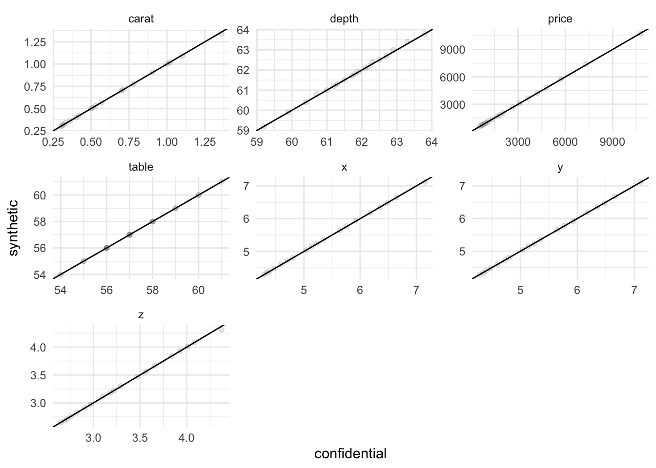
7 depth    kurtosis     2.56      3.27      0.709                 0.277 

We also look at important percentiles.

eval_data <- bind_rows(
  "confidential" = diamonds_prepped,
  "synthetic" = synth1$synthetic_data,
  .id = "source"
)  

eval_data %>%
  select(source, where(is.numeric)) %>%
  group_by(source) %>%
  summarize(
    quantile = seq(0.05, 0.95, 0.05),
    across(everything(), .fns = ~quantile(.x, probs = seq(0.05, 0.95, 0.05)))
  ) %>%
  ungroup() %>%
  pivot_longer(
    c(-source, -quantile), 
    names_to = "variable", 
    values_to = "value"
  ) %>%
  pivot_wider(names_from = source, values_from = value) %>%
  ggplot(aes(confidential, synthetic)) +
  geom_abline(intercept = 0, slope = 1) +
  geom_point(alpha = 0.1) +
  #coord_equal() +
  facet_wrap(~ variable, scales = "free")

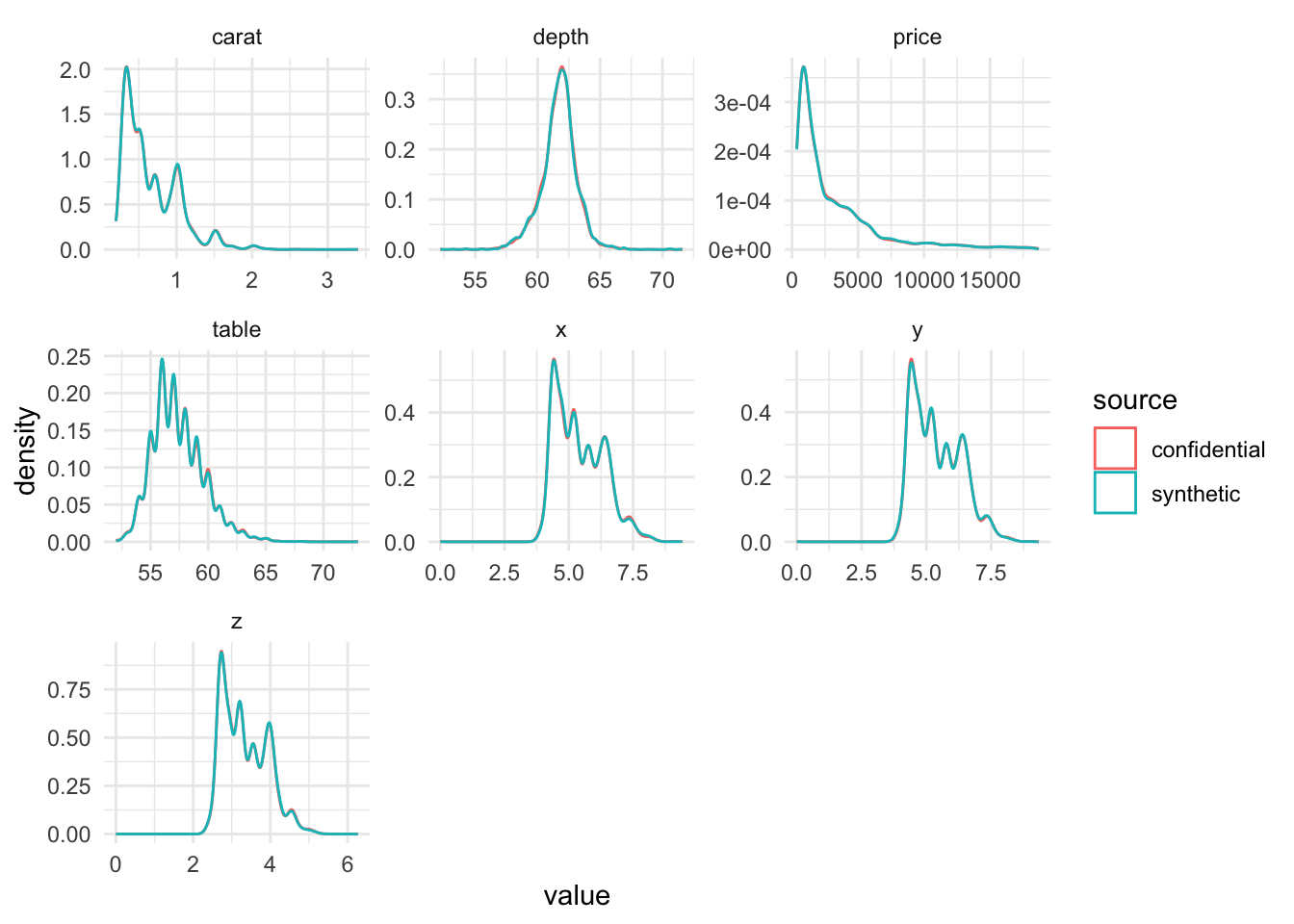
We look at density plots. The original data and synthetic data have comparable distributions for all variables.

eval_data %>%
  select(source, where(is.numeric)) %>%
  pivot_longer(-source, names_to = "variable", values_to = "value") %>%
  ggplot(aes(value, color = source)) +
  geom_density() +
  facet_wrap(~ variable, scales = "free")

9.3.2 Multivariate

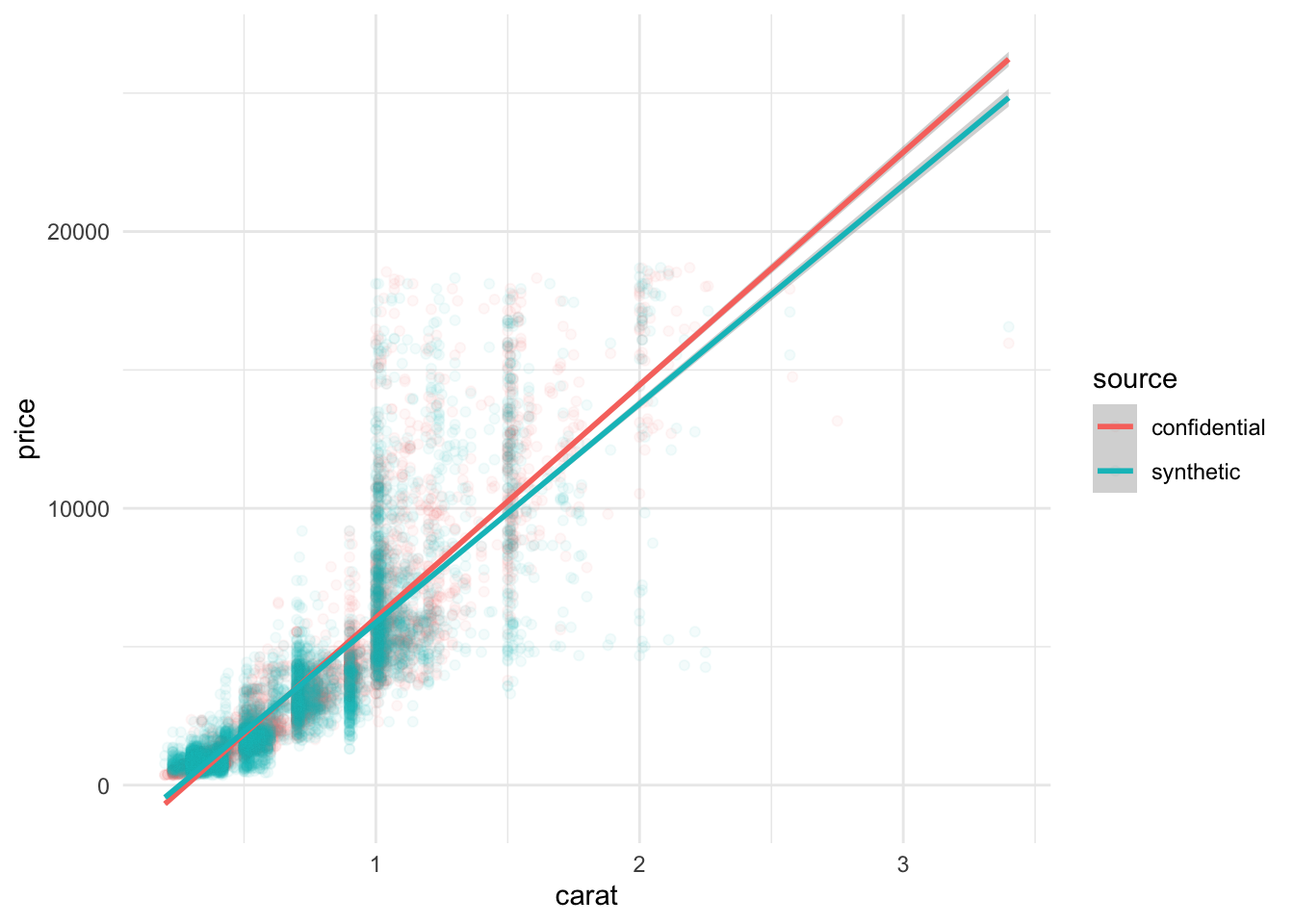
We look at a few key relationships. It is difficult to distinguish between the original data and synthetic data.

eval_data %>%
  ggplot(aes(carat, price, color = source)) +
  geom_point(alpha = 0.05) +
  geom_smooth(method = "lm")

`geom_smooth()` using formula = 'y ~ x'

We look at how well the synthetic data recreate the correlations in the original data.

util_corr_fit(
  synth1, 
  diamonds_prepped
)$correlation_difference_mae

[1] 0.04581184

This means that the average correlation difference is off by about 0.05 in the synthetic data.

util_corr_fit(
  synth1, 
  diamonds_prepped
)$correlation_difference %>%
  round(digits = 2)

      carat     x     y     z price table depth
carat    NA    NA    NA    NA    NA    NA    NA
x     -0.04    NA    NA    NA    NA    NA    NA
y     -0.05 -0.03    NA    NA    NA    NA    NA
z     -0.04 -0.03 -0.04    NA    NA    NA    NA
price -0.05 -0.05 -0.06 -0.04    NA    NA    NA
table -0.05 -0.04 -0.04  0.00 -0.01    NA    NA
depth  0.01  0.06  0.05 -0.06  0.02  0.19    NA

The errors are pretty even across the correlation matrix.

disc1 <- discrimination(postsynth = synth1, data = diamonds_prepped)

rpart_rec <- recipe(
  .source_label ~ ., 
  data = disc1$combined_data
)

rpart_mod <- decision_tree(cost_complexity = 0.001) %>%
  set_mode(mode = "classification") %>%
  set_engine(engine = "rpart")

disc1 <- disc1 %>%
  add_propensities(
    recipe = rpart_rec,
    spec = rpart_mod
  ) 

disc1 <- disc1 %>%
  add_pmse %>%
  add_pmse_ratio(times = 100)

disc1$pmse

# A tibble: 2 × 4
  .source  .pmse .null_pmse .pmse_ratio
  <fct>    <dbl>      <dbl>       <dbl>
1 training 0.140     0.0115        12.3
2 testing  0.141     0.0114        12.3

The pMSE ratio is a discriminant-based metric. The value of the pMSE ratio is good but not great in this case.

9.4 Approach #2

We create a second synthesis. This time, we add extra noise to predicted values when synthesizing the data. Fortunately, we can reuse many of the objects created in the first synthesis. Here, we update the noise object and the presynth object. Then we synthesize again.

We add extra noise to our predicted values. We use 400 ntiles, which works out to about 17 observations per ntile.

noise2 <- noise(
  roadmap = roadmap,
  add_noise = TRUE,
  ntiles = 400
)

presynth2 <- presynth(
  roadmap = roadmap,
  synth_spec = synth_spec,
  noise = noise2,
  constraints = constraints,
  replicates = replicates
)

synth2 <- synthesize(presynth2)

The original data has limited precision. We round the synthetic variables to match this precision.

synth2$synthetic_data$table <- round(synth2$synthetic_data$table, digits = 0)
synth2$synthetic_data$carat <- round(synth2$synthetic_data$carat, digits = 2)
synth2$synthetic_data$y <- round(synth2$synthetic_data$y, digits = 2)
synth2$synthetic_data$x <- round(synth2$synthetic_data$x, digits = 2)
synth2$synthetic_data$z <- round(synth2$synthetic_data$z, digits = 2)
synth2$synthetic_data$price <- round(synth2$synthetic_data$price, digits = 0)
synth2$synthetic_data$depth <- round(synth2$synthetic_data$depth, digits = 1)

Most of the utility metrics look comparable to the first synthesis; however, the pMSE ratio increases modestly.

disc2 <- discrimination(postsynth = synth2, data = diamonds_prepped)

rpart_rec <- recipe(
  .source_label ~ ., 
  data = disc1$combined_data
)

rpart_mod <- decision_tree(cost_complexity = 0.001) %>%
  set_mode(mode = "classification") %>%
  set_engine(engine = "rpart")

disc2 <- disc2 %>%
  add_propensities(
    recipe = rpart_rec,
    spec = rpart_mod
  ) 

disc2 <- disc2 %>%
  add_pmse %>%
  add_pmse_ratio(times = 100)

disc2$pmse

# A tibble: 2 × 4
  .source  .pmse .null_pmse .pmse_ratio
  <fct>    <dbl>      <dbl>       <dbl>
1 training 0.148     0.0116        12.7
2 testing  0.147     0.0116        12.6

• add hyperparameters
• add evaluation
• add constraints