18  Using Non-Point Resource Data: Baltimore Capital Improvement Program

Every year, Baltimore City adopts a capital budget with millions of dollars set aside to repair and improve public resources like sewer lines, water mains, roads, bridges, and public buildings. Unfortunately, like many older US cities, Baltimore City rarely has sufficient funding to meet all of the city’s public infrastructure needs.

How can we make sure that neighborhoods across the city get their fair share?

This case study shows how the Baltimore City Department of Planning staff are using the Urban Institute’s Spatial Equity Data Tool and sedtR R package to create a reproducible analysis of Department of Transportation capital investments. The study includes both a limited introduction to the process of analyzing a capital program and a basic overview of how to use the sedtR package in combination with other popular R packages for data wrangling and visualization.

This case study also shows off the new arcgislayers package (part of a new collection of R packages for working with the ArcGIS ecosystem) to access GIS data published online. Preparing and visualizing the data also use the popular sf R package and tidyverse package family.

Case and Policy Background

The Baltimore City Department of Planning (the agency that oversees the development of the City’s annual Capital Improvement Program (CIP)) conducts a spatial analysis to understand where the investment is going and how the demographics of the areas that receive investment compare to the city as a whole. This work started in 2017 when the Department of Planning (DOP) developed an Equity Action Plan with five key goals—including using an equity lens to prioritize the city’s capital investments. In 2018, the plan became law when Baltimore City Council adopted the city’s Equity Assessment Ordinance (or Equity Ordinance for short) requiring that the agency complete an equity assessment of the annual capital budget.

The Baltimore Neighborhood Indicators Alliance at the University of Baltimore developed the city’s existing approach (described in detail in this August 2019 report). DOP staff have continued to use this model to create a new report on each year’s budget. This analysis uses spatial data on capital projects shared by agency staff as part of the annual process of developing the Capital Improvement Program and capital budget. Following the adoption of the capital budget, many agencies also publish data on active capital projects to support web maps and applications.

Why Use the SEDT

This existing equity analysis, however, has some key limitations. The analysis process involves assigning “weights” to projects and assessing the weighted distribution of capital projects across neighborhoods. However, this assignment is largely subjective, and the process to execute the analysis in ArcGIS Pro is entirely manual. As a result, the analysis is only completed a few times per year and is provided to agencies after recommendations for the Capital Improvement Program are near final.

The Spatial Equity Data Tool has the potential to improve this process by making it faster and easier for city staff to complete an equity analysis and for agency staff to using this information in preparing equitable budgets.

In addition to demonstrating the sedtR package, this case study also shows off the new arcgislayers package (part of a new collection of R packages for working with the ArcGIS ecosystem) to access GIS data published online. We also use the popular sf R package and tidyverse package family for preparing and visualizing the data.

About the Data

For this case study, the Department of Planning selected capital projects by the Baltimore City Department of Transportation as an initial focus. As one of the most visible elements of the city’s infrastructure, the physical condition of Baltimore’s street network is a consistent topic of interest for both the public and local elected officials.

Within the Department of Transportation (DOT), capital planning is divided among the agency’s divisions and groups. The Transportation Engineering and Construction (TEC) Division manages most capital improvement projects: road reconstruction and resurfacing projects are led by the Highways and Streets Engineering Group along with other groups focused on alleys, footways, and bridges.

Following the development of the Complete Streets Manual in 2021, DOT has sought to apply the Project Prioritization Process outlined in the manual to inform requests for future capital projects. The agency’s 2024 presentation to the Planning Commission explained how this process emphasized “equity…as a leading factor followed by asset condition and safety, with a reduced focus on complaint driven projects and the equal spreading of projects based on geographic/council boundaries.”

Since 2019, the Department of Transportation has published an interactive web map with the location of planned, under construction, and completed resurfacing projects. The map builds on an existing initiative, Project Orange Cone, that has published information on street resurfacing since 2007.

For purposes of this case study, Department of Planning staff created a reference copy consolidating all of the 2019 to 2024 resurfacing data into a single layer. We can use the arcgislayers::arc_read() function to read this data into R:

# If you need to install sedtR:
#install.packages("devtools")
#devtools::install_github("UrbanInstitute/sedtR")

# Load relevant packages for the analysis:
library(sedtR)
library(arcgislayers)
library(sf)
library(tidyverse)
library(tmap)

dot_resurfacing <- arc_read(
  "https://services1.arcgis.com/43Lm3JYE3nM91DAF/arcgis/rest/services/BCDOT_Resurfacing_Program_Locations/FeatureServer/0",
  crs = 3857
)

For context, we can also download the boundaries of the sectors used by the agency to divide up resurfacing and other programs:

dot_sectors <- arc_read(
    "https://services3.arcgis.com/ZTvQ9NuONePFYofE/arcgis/rest/services/Transportation_Sector_Boundaries/FeatureServer/0",
    crs = 3857
)

Now, we can take a look at the program’s 2023 data to show what a typical year of resurfacing projects looks like:

dot_resurfacing |> 
  filter(
    year == "2023"
  ) |> 
  rename("Project Status" = status) |>
  ggplot() +
  geom_sf(data = dot_sectors, fill = NA, linewidth = 1.5) +
  geom_sf(aes(color = `Project Status`), linewidth = 1.5) +
  scale_color_brewer(palette = "Dark2") +
  labs(
    title = "Baltimore City Resurfacing Projects, 2023",
    caption = "Note: Grey lines indicate DOT Sectors\nSource: Baltimore City Department of Transportation"
  ) +
  theme_void() +
  theme(plot.caption = element_text(hjust = 0))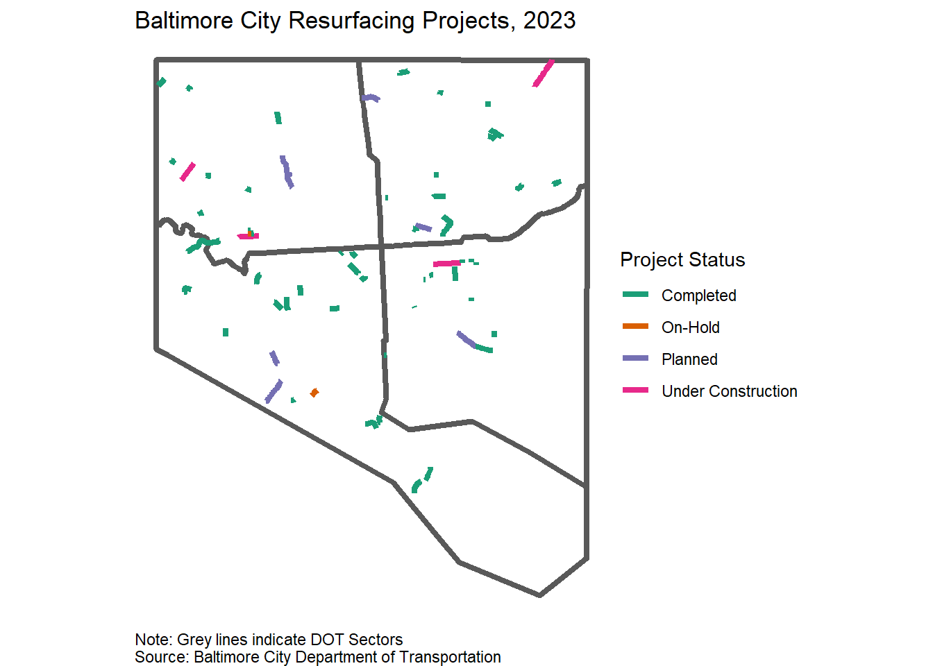

Each year, DOT uses program funds to repave different road segments. To ensure the analysis is representative of the overall coverage, we decided to include completed locations for the full five years available:

completed_resurfacing <- dot_resurfacing |> 
  # Filter to completed resurfacing segments
  filter(status == "Completed")

Applying the SEDT to the Department of Transportation Resurfacing Program

This case study analyzes the Baltimore City Resurfacing Program that is part of the Capital Improvement Program (CIP). We include three sections that explore how to use the CIP project location data in combination with the SEDT API:

• Preparing input data
• Making a call to the SEDT API
• Visualizing and interpreting results

Note that this analysis is not a formal determination of spatial equity by the department and has a number of key limitations that are not fully explored in this case study. It is presented largely to improve the Baltimore Department of Planning’s understanding of how to use and apply this new approach and, more broadly, to serve as a possible use case for the SEDT.

Preparing input data

Since the Spatial Equity Data Tool is designed for use with point data, using project locations made of lines posed a challenge. To address this, we decided to convert the data into points but preserve the length of the street segments within each Census tract as a weighting variable.

Using the sf package and the tigris package, the process follows:

• Downloading Census tract boundary data using the {tigris} R package or some other source
• Intersecting the input data with the tract geography using sf::st_intersection()
• Calculating a resource weight column based on length calculated with sf::st_length()
• Converting the geometry from lines to points using sf::st_point_on_surface()

# Download tract data for Baltimore City
baltimore_tracts <- arc_read(
  "https://services1.arcgis.com/UWYHeuuJISiGmgXx/ArcGIS/rest/services/Census_Tract_2020/FeatureServer/0",
  crs = 3857
) |> 
  # Transform to match input data CRS
  st_transform(st_crs(completed_resurfacing))

resurfacing_weighted <- completed_resurfacing |> 
  # Intersect with tracts
  st_intersection(select(baltimore_tracts, geometry)) |> 
  # Get length of new segments
  mutate(
    length = as.numeric(st_length(geometry)),
    .before = geometry
  ) |> 
  # Convert to points
  st_point_on_surface() |> 
  suppressWarnings()

Using weighted points allows the resource data to better represent how road resurfacing projects work. If a resurfacing project is beneficial for area residents, the benefit can be measured based on the length of the resurfacing. We also explored using un-weighted data or weighting by area (after applying a small buffer to each segment) but determined that weighting by length worked best among these options.

Making a call to the SEDT API

After preparing the data, it is easy to pass the sf object to the API using call_sedt_api(). We must set the resource_weight argument to the length variable created in the code chunk above in order to use the weighting variable we just calculated.

Note that call_sedt_api() can take a number of input data types as an object (using the resource argument) or as a path to the data file (using the resource_file_path argument):

• A sf or sfc object with POINT geometry as shown below (resource argument)
• A URL for a delimited file with coordinate columns or a spatial data file (resource_file_path argument)
• An ArcGIS FeatureLayer or Table URL (resource_file_path argument)
• A file path to a delimited file with coordinate columns or a spatial data file on the user’s local computer (resource_file_path argument)
• A data.frame object containing the named columns in coords (resource argument)

resurfacing_resp <- call_sedt_api(
  resource = resurfacing_weighted,
  resource_weight = "length"
)

The API returns a list with two key components: geo_bias_data and demo_bias_data. This data enables us to visualize and map the spatial equity aspects of the program locations.

glimpse(resurfacing_resp)

Visualizing and interpreting results

The sedtR package provides two built-in functions for visualizing and mapping results: create_demo_chart() and create_map().

First, we can use the create_demo_chart() function to create a “lollipop” plot of the data with ggplot2. This helps us look at the demographic bias data showing whether the population subgroups in areas where resurfacing projects take place are over- or underrepresented relative to Baltimore City’s population overall. For example, if resurfacing projects only took place in the wealthiest sections of the city, people under the poverty line may be underrepresented in this analysis.

The resulting plot shows that Hispanic Baltimore residents and residents who have not attained a high school diploma are both overrepresented in the data. The percentage of population with a bachelor’s degree and the percentage of renter households are both underrepresented.

resurfacing_resp |> 
  pluck("demo_bias_data") |> 
  create_demo_chart()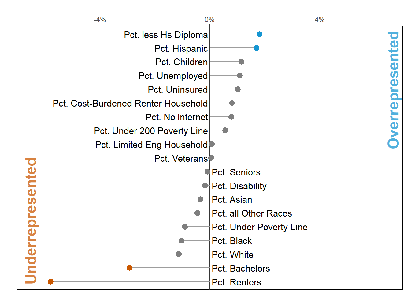

The finding that renters are underrepresented is unsurprising; many renters live in small, downtown census tracts that likely have fewer streets relative to larger census tracts. More generally, the scale of the demographic disparity score differences is small, and most of the differences are not statistically significant. In addition, one of the two underrepresented groups is people who hold bachelor’s degrees—- a traditionally advantaged group when compared with individuals with less educational attainment. This result suggests that the resurfacing program may already be effective at distributing investment evenly across the city’s neighborhoods and demographic groups.

Next, we can use the create_map() function, which utilizes the tmap package to map the geographic disparity scores.

resurfacing_resp |> 
  pluck("geo_bias_data") |> 
  create_map()

The map shows whether the input resource is over- or underrepresented relative to the share of the city’s overall population living within the tract. For example, if 5 percent of the city’s population lived in one tract, we might expect 5 percent of resurfacing work to take place in that area.

However, the area with the longest roads (and potentially greatest need for resurfacing) may not have the largest number of residents. For example, in the larger tracts in south, southeast, and southwest Baltimore stand out with higher disparity scores (>2 percent). These areas have long roads but smaller populations compared with small, dense tracts in downtown and central Baltimore.

Some of these same areas are also close to the major arterial roads that connect the city’s industrial areas to local highways. A larger number of heavy vehicles can cause more damage to pavement requiring more frequent and extensive resurfacing work to maintain.

To get a better look at other factors, such as volume of traffic, we can also examine the MDOT SHA Annual Average Daily Traffic (again using arcgislayers to access the data). The map below shows roads in the 90th percentile or above in terms of 2022 Baltimore City traffic volume. The overlap of many of these roads with blue census tracts illustrates how the city may focus on resurfacing heavily used roads.

baltimore_aadt <- arc_read(
      "https://services.arcgis.com/njFNhDsUCentVYJW/ArcGIS/rest/services/MDOT_SHA_Annual_Average_Daily_Traffic/FeatureServer/1",
      where = "COUNTY_DESC LIKE 'Baltimore City'",
      crs = 3857
  ) 

top_10_percentile <- baltimore_aadt |>
  pull(AADT_2022) |>
  quantile(0.9, na.rm = TRUE)

baltimore_top_aadt <- baltimore_aadt |>
  filter(AADT > top_10_percentile)

if (rlang::is_installed("urbnthemes")) {
  pal <- urbnthemes::palette_urbn_diverging
} else {
  pal <- "RdBu"
}

processed_geo_data <- resurfacing_resp$geo_bias_data |>
  mutate(diff_pop = ifelse(sig_diff_pop == "FALSE",
                           NA,
                           diff_pop * 100))


map <- tm_basemap("CartoDB.PositronNoLabels") +
tm_shape(processed_geo_data,
         name = "Geographic Disparity Scores") +
  tm_fill(col = "diff_pop",
          palette = pal,
                midpoint = 0,
                legend.show = TRUE,
                id = "id_col",
                title = "Disparity Score",
          textNA = "Not Stat. Sig.",
          legend.format= list(
                  fun=function(x) paste0(formatC(x, digits=1, format="f"), " %")
                  ),
          alpha = .5) +
  tm_borders(alpha = .05) +
  tm_shape(baltimore_top_aadt,
           name = "Most Travelled Roads (2022)") +
  tm_lines(lwd = 2.5,
           col = "black",
           legend.lwd.show = TRUE, legend.col.show = TRUE,
           legend.show = TRUE) +
  tm_layout(title = "Most Travelled Roads (2022)") +
  tmap::tm_tiles("CartoDB.PositronOnlyLabels")

map

Overall, the resurfacing program does not have a clear pattern of demographic or spatial disparities. The extent of the five-year period used for the input data may have contributed to this finding, but looking at each year individually seemed to introduce a different set of challenges. As the Department of Transportation continues to adjust programs based on the equitable project prioritization process, these results may change to show greater investment in areas occupied by historically disadvantaged groups. Given the limited scope of this investigation, more research is required for a full understanding of the reasons behind the results.

Conclusion

The Spatial Equity Data Tool is a promising resource for local governments interested in exploring the potential of reproducible methods as a way of investigating the spatial equity of capital programs. Key elements of our approach so far have included the following:

• Combining data from multiple years to avoid skewing results
• Preparing non-point data using an appropriate method specific to the asset type
• Visualizing SEDT API responses together with alternate data sources

We plan to continue using the tool to develop applications for other city programs or capital asset types. If you are another sedtR user, please get in touch to share your approach so we can learn how to use these tools together.