19 Conducting Analyses with Travel Sheds
This feature is only available in the API.
Urban introduced a beta version of the travel shed functionality into the tool in early 2025. The functionality is being tested and is available at the county and city scale for datasets in the District of Columbia, Virginia, and Maryland. Urban hopes to expand the functionality to all states soon.
At the time of this release in February, 2025, Urban is aware that the walk sheds in three Virginia tracts were erroneously calculated and are too large. We believe this result stems from our workaround to ensure we are able to create a polygon in every tract. We describe this approach in detail in our blog, but, in short, it ensures we are able to create sheds even in rural and remote census tracts.
As we expand and build off of this beta functionality, we plan to address this issue.
The FIPS codes of the three tracts are: 51153901504, 51001090202, and 51001090201. These tracts fall within Virginia’s Prince William and Accomack counties, so analyses in these counties will be affected. These tracts fall outside of all cities in the tool, so city scale analyses will be unaffected. This issue could impact analyses by falsely determining points outside of walking distance from those tracts are actually accessible to them, leading the tool to deem there to be disproportionately high over–representation in these tracts.
Background and Introduction to Travel Sheds
A travel shed is a polygon that reflects all the areas accessible under a specified amount of time using some mode(s) of transportation from some point. At a high level, the travel shed functionality in the tool allows users to choose whether to define a resource as accessible to the residents of a tract if it is within a given walk or drive time of the center of a census tract instead of defining access as whether the resource is within the tract itself.
The Census Bureau defines census tracts as “small, relatively permanent statistical subdivisions of a county” with similar populations (between 1,200 and 8,000, averaging 4,000). As a result, they can vary significantly in size, with tracts in more densely populated urban areas being much smaller than tracts in less densely populated rural areas.
Before the introduction of travel sheds into the SEDT, the tool deemed all points outside of a census tract as inaccessible to it. In many cases, the census tract a resource falls into can be a reasonable approximation of the area it serves. For example, resource datasets reflecting 311 call requests, Wi-Fi hotspots, playgrounds, street lights, pothole repairs, access ramps, or fire hydrants could all reasonably be deemed to provide a service to the residents of the census tract where they are located, making the tool’s traditional conceptualization (which we’ll refer to as the “standard SEDT analysis” throughout this chapter) useful for these resource data.
However, some resources provide services to areas materially different from the tract in which they are located. As one example, consider trauma centers in the city of Chicago, Illinois. Chicago has hundreds of census tracts but only six hospitals with trauma centers. A trauma center is a part of a hospital that provides specialized care to patients suffering from acute and severe traumatic injuries. The standard SEDT analysis of trauma centers in Chicago would show the five census tracts where the trauma centers are located (two trauma centers are in the same tract) as being highly overrepresented in their access to trauma centers, while all other tracts are underrepresented. This does not reflect how these hospitals serve broader regions of the city and suggests that a different approach to access could be useful.
We reviewed the spatial access literature and conducted substantial user engagement when considering how to expand the tool to address this challenge. Based on these conversations, we determined travel sheds to be the most useful method of the approaches we considered. These conversations also guided the specific modes and time thresholds we chose to develop. For more details on the process of selecting these travel modes and times, please see our blog post announcing the travel sheds.
Travel Shed Options
The tool allows users to choose six different specifications:
- Walk shed:
- 10 minutes
- 15 minutes
- 20 minutes
- Drive shed:
- 15 minutes
- 30 minutes
- 60 minutes
For every census tract, the six travel sheds listed above were calculated starting from a central point in the tract. In the majority of cases, we used the population-weighted centroid. When we were not able to use the population-weighted centroid, we used a central point in the tract or, if that did not work, a randomly selected point. See our blog post for more details.
Once a user selects a travel shed, the tool conducts its calculations using them. The tool treats all points within the travel shed as accessible to the census tract.
Creating the Travel Sheds
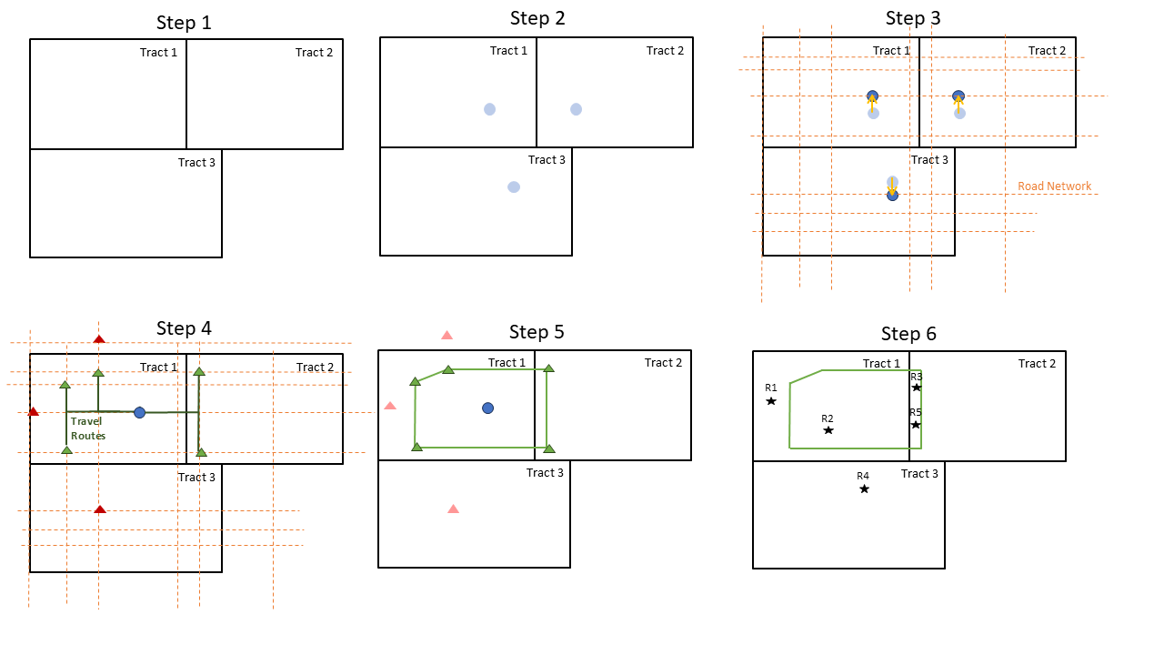
The diagram above illustrates our method for creating travel sheds. Let’s consider a geography with three tracts (step 1). We use Census Bureau data to identify the population-weighted centroid of each tract, shown as blue circles in step 2. Due to higher population density near the intersection of the three tracts, these centroids are closer to that intersection in our example. Next, we snap the population-weighted centroids with the nearest street network, represented by dotted orange lines in step 3. We then calculate the distance to street network vertices (intersections) and determine the vertices with the largest travel time for the specified travel shed. This is demonstrated for tract 1 using green triangles in step 4. We connect these points to form a concave polygon, creating a travel shed, shown as the green polygon in step 5. Although we apply these steps to all tracts, we only illustrate steps 4 and 5 for tract 1 for clarity. Finally, we assess the number of points within the travel shed for a given point as shown in step 6.
This example shows how a travel shed approach differs from the standard SEDT approach. While resource 1 is accessible to tract 1 in the standard SEDT approach, it is not with the travel shed approach. Resource 2 is accessible to tract 1 in both approaches. Resources 3 and 5 are accessible in the travel shed approach but not in the standard SEDT approach. Resource 4 is inaccessible in both approaches. While this is a stylized example, all of these possibilities are possible when using travel sheds with the tool.
We used the r5r R package to handle steps 3–5 of the process above. We accessed the population-weighted census tract data via IPUMS NHGIS (Manson et al. (2024)).
For more details about this process, see our blog post. In particular, it outlines what we do when we are unable to snap a population-weighted centroid to the road network (step 3) and if we do not have enough points to create a polygon (step 5). The latter workaround likely results in the bug we described in the callout note at the top of this page.
When and Why Users Should Use Travel Sheds
The tool currently allows the usage of travel sheds at the city and county scales. We are hopeful to release state- and national-level scales at a later date.
Users should decide whether to use travel sheds based on the resource data itself and the population in the geography where that data is located. We recommend asking the question “Does this resource serve an area larger than the census tract in which it’s located?” If the answer is “yes,” then using travel sheds may be appropriate.
Once a user decides to use travel sheds, the next question is whether a drive shed or a walk shed is more appropriate. Here, we recommend asking the question, “what mode will most people in my focus geography use to access the resource?” For some highly specialized and scarce resource datasets (e.g., hospitals), residents likely access them by car regardless of where they live. In this case, using a drive travel shed is likely the most appropriate choice.
For other resource datasets, residents’ approach to accessing them likely varies by location. For example, in dense urban areas, residents likely often walk to elementary schools, supermarkets, and polling places, so using walk sheds would be most appropriate. In more rural areas, residents may more often drive to these same locations, making the drive sheds the most appropriate choice.
Once the user selects the mode of travel, they should then select the travel time limit to use for the shed. We recommend asking the question, “How long is it reasonable for people to travel to access this resource to be considered to have meaningful access?” For example, in urban areas, it is likely unreasonable to expect that people would drive 30 minutes to access a grocery store, and a shorter drive time would be more appropriate. But it may be more reasonable to expect that individuals would drive 30 minutes to access a job-training site in a county with a small number of sites.
If a user is unsure of how residents will access a given resource, they can try both modes or multiple time thresholds to understand how such changes affect access to resources. For resources that roughly serve the census tract in which they are located, using the standard SEDT analysis is the best choice.
Interpreting the Disparity Scores
Geographic disparity scores for travel shed analyses
Travel shed analyses are currently available at the city and county scales for geographies within Virginia, Washington DC, and Maryland.
For a travel shed analysis, the geographic disparity score for a given tract is the difference between the proportion of user-uploaded data within the travel shed associated with a census tract and the proportion of the tract’s baseline population within the tract.
Consistent with the standard SEDT analysis, the geographic disparity scores calculated with travel sheds tell us whether the baseline population within the tract is over- or underrepresented in their access to the data. However, in this case, access is not determined by a tract boundary but rather by the boundary of a user-selected travel shed associated with the tract. For example, in a county-level analysis using 15-minute car travel sheds, if a tract had a geographic disparity score of 1.2, that would mean that the share of data within the 15-minute drive travel shed associated with the tract was 1.2 percentage points higher than the share of the baseline population in the tract.
Demographic disparity scores for travel shed analyses
Demographic disparity scores for travel shed analyses represent the percentage point difference between the representation of a demographic group in areas that can access the locations of the uploaded data (the data-implied percentage) and the representation of that group in the geography (the geography-wide percentage). For a travel shed analysis, we define the areas that can access the locations of the uploaded data as those tracts where the uploaded points fall within the tract’s travel shed, not the tract’s boundaries. Like the demographic disparity score outside of the travel shed context, positive disparity scores mean that a demographic group makes up a larger share of the population in tracts with access to the original data than the geography as a whole. Negative disparity scores mean that a demographic group makes up a smaller share of the population in tracts with access to the data than the geography as a whole.
Understanding Travel Shed Results
As noted in Chapter 12, there are two major differences in how the tool functions when using travel sheds. First, points can be deemed accessible to the residents of multiple census tracts because travel sheds can extend beyond tract boundaries and can overlap with each other.
Second, the tool does not filter points. The standard SEDT analysis filters user-uploaded data only to include the points that fall within the target geography. For example, if a user selects county-level analysis and uploads a dataset with points in multiple counties, the tool will perform the analysis on the county with the largest number of points and drop all points falling outside that county. See Chapter 12 for details. The travel shed analysis keeps all points in the user-uploaded data as the travel shed approach can consider points outside of a given geography accessible to tracts within that geography. As a result, users should filter their data only to include resources that legitimately serve or impact residents of the geography or that they view should serve or impact residents of the geography.
As a consequence of these changes, using the tool with travel sheds moves away from a “relative” level of access. In standard SEDT analyses, for the geographic disparity score, if one sub-geography had a higher proportion of the data points relative to the baseline population, then some other sub-geography must have had a lower proportion of the data points relative to the baseline population. Similarly, for the demographic disparity score, if one demographic group had a higher representation in the data-implied percentage, then some other demographic group likely would have a lower representation in its data-implied percentage. However, with travel sheds, this is not necessarily the case. Multiple tracts with different demographic compositions can access the same set of points, and some points may not fall within any travel sheds.
This change for travel sheds unlocks the tool’s ability to provide new insights about service provision of uploaded resources, but users must also create tool requests carefully. In particular, they should consider results showing uniform over- or underrepresentation carefully. We provide more details on each of these two ideas in the sections below.
All the geographic and/or demographic disparity scores are overrepresented
As discussed above, census tracts are designed to have similar amounts of people in them, but, as a consequence, they vary dramatically in size. Car travel sheds tend to be far larger than census tracts, particularly in urban areas.
If a user uses car travel sheds, especially for a dense city or county, it would be unsurprising that the vast majority of tracts in the geographic disparity score and groups in the demographic disparity score are “overrepresented” as many tracts will be able to reach a greater share of points within the car travel time than the share of the baseline population residing in the tract. If a user sees such results, they should consider whether the travel shed is appropriate. If they have selected a travel time that is longer than it would be reasonable to expect residents to travel to reach the resource, they should consider updating their analyses with a more appropriate travel time choice, which could mean selecting a shorter travel time, using walk sheds, or using the standard SEDT analysis. If the user deems that the travel time and mode are appropriate, this result suggests that residents have high access to the given resource.
All the geographic and/or demographic disparity scores are underrepresented
Walk travel sheds or small drive sheds may be smaller than census tracts, and this is almost certainly true in rural counties and small, less-dense cities. If a user analyzes a more rural area, particularly with walk sheds, it is possible that many resources within the geography may be outside of all travel sheds. If this is the case, most demographic and geographic disparity scores would show underrepresentation. If a user sees such results, they should consider whether the travel shed is appropriate. If they have selected a travel time or travel mode that does not align with reasonable expectations for how residents access a given resource, they should consider updating their analyses with a more appropriate travel time choice, which could mean selecting a longer travel time, using drive sheds, or using the standard SEDT analysis. If the user deems that the travel time and mode are appropriate, this result suggests that residents have low access to the given resource. Again, we flag the warning that, unlike using the tool without travel sheds, no points outside of the geography are dropped.
Using Travel Sheds with the API
To specify a travel shed, change the value of the "distance_access" parameter in the API request from null (the default) to one of the following six alternatives:
{“walk”: 10}{“walk”:15}{“walk”:20}{“drive”:15}{“drive”:30}{“drive”:60}
Only analyses conducted at the city or county scale in Washington, DC, Virginia, and Maryland can be run using travel sheds at this time. For this beta release, we have started with these three states for testing, but we hope to expand the functionality to all geographies soon.
Limitations
Sheds calculated from a central point
Travel sheds are calculated from a single origin point and estimate the universe of locations that can be reached from the origin point by the specified travel mode and within the specified time limit. To make the calculation of the sheds computationally feasible, we represent the travel shed for a given census tract using the travel shed calculated from a single point (most often the population-weighted centroid) of the tract. This essentially introduces the simplifying assumption that all residents in a census tract live at that population-weighted centroid.
As discussed above, census tracts are designed to have similar amounts of people in them, but, as a consequence, they vary dramatically in size. Consequently, the distance between a resident’s true location and the population-weighted center of a census tract varies based on tract size. In small, dense tracts, this distance is almost always low, which means that the loss of precision from the simplifying assumption of using the population-weighted centroid to represent the whole tract is low. However, in rural areas, it is possible that there is a meaningful distance between the population-weighted center of a tract and a resident’s true location. This could result in a more significant loss of precision in applying the simplifying assumption in rural areas.
Users should recognize that the sheds are calculated from a single, central point for a given census tract and can very effectively reflect access for residents living close to that point. Users should recognize that these analyses will not perfectly capture access for residents living far from the central point of a tract, which may have a more significant impact on analysis results in rural or less densely populated urban or suburban areas.
Sheds calculated at single time of day and with single mode
The travel sheds are calculated using a single mode of transportation (walking or driving). Other transportation modes, like using mass transit or a bicycle, are not available, nor is the possibility of multimodal travel. In addition, the r5r package does not account for traffic when calculating drive times. In reality, travel times vary substantially throughout the day due to traffic. For resources that are commonly accessed at high-traffic times of day, such as schools or workplaces, users should be aware that the travel sheds likely overestimate distances that could be traveled in traffic, especially in urban areas.
In the future, we hope to explore the possibility of a traffic multiplier and expand the number of modes included.
Jagged sheds
As noted in our blog post, we created isochrones using the r5r R package which itself calls the concaveman R package. A key component of this approach is identifying a set of destination points and the time it takes to travel to those points. More specifically, the r5r package selects destination points from the intersections of a road network dataset provided to the function. The software calculates the travel time to each destination point. Then r5r uses the concaveman R package to interpolate them into a concave polygon representing the travel shed (you can see the difference between concave and convex polygons in this blog post). In other words, r5r “connects the dots” of the destination points to make a travel shed polygon.
This process has a few limitations. First, in our testing, it appears that r5r is somewhat inconsistent in its choice of destination points. Second, as noted in the blog post, sometimes, there are too few destinations in the road network, and we added additional nearby destination points for walk sheds to make the code run successfully. Lastly, the concaveman algorithm itself results in jagged polygons. These issues all matter because the borders of the travel sheds represent the travel frontier, but they may not capture this edge perfectly. As a consequence, in literal edge cases, the tool may incorrectly determine that a resource point is or is not accessible to a travel shed due to this imprecision.
As we continue to develop this work, we hope to test further how our solution for remote census tract centers with few nearby destination points impacts the degree to which the polygons are jagged. We also hope to explore this process more generally to expand the results.