| Population MOE | White resident MOE | |
|---|---|---|
| Tract A | 5.5 | 5.0 |
| Tract B | 3.5 | 1.5 |
14 Statistical Significance Calculations
To calculate the statistical significance of our demographic and geographic disparity scores, we make use of several Census-provided standard error and margin of error formulas (US Census Bureau 2020). We use Equation 14.1 for aggregating data across geographic areas:
\[ MOE(\hat{X}_1 + \hat{X_2} + ... + \hat{X_n}) = \\ \pm \sqrt{[MOE(\hat{X_1)}]^2 + [MOE(\hat{X_2})]^2 + ... + [MOE(\hat{X_n})^2])} \tag{14.1}\]
and Equation 14.2 for computing standard errors and margins of error of user-derived percentages:
\[ MOE(\hat{P}) = \frac{1}{\hat{Y}} \sqrt{[MOE(\hat{X})]^2 - (\hat{P^2} *[MOE(\hat{Y})]^2)} \tag{14.2}\]
For the rest of this section, we will refer to these formulas as Equation 14.1 and Equation 14.2. Since we are interested in computing standard errors, we will also make use of the fact that:
\[ SE(X) = \frac{MOE(X)}{1.645} \]
Geographic Disparity Scores
The geographic disparity score is the percentage point difference between the proportion of the data originating in a subgeography (state for national-level analysis, county for state-level analysis, and tract for county- and city-level analysis) and the proportion of a geography’s total baseline population (total population, child population, etc.) residing within a subgeography. The proportion of the data originating from a subgeography (the data proportion) is a fixed number, but the proportion of a geography’s total baseline population residing in a subgeography (baseline proportion) is an estimate from the ACS five-year survey, with associated margins of error for both the numerator (the total baseline population in the subgeography) and the denominator (the total baseline population in the geography). To take into account the variability in the ACS measures, we computed standard errors for the baseline proportions using Equation 14.1 and Equation 14.2 to construct 95 percent confidence intervals for the geographic disparity score. If the confidence interval contains 0, then we report that subgeography’s disparity score as insignificant.
As a simple example, imagine a geography with two census subgeographies, A and B. Subgeography A contains 20 people and 10 data points. Subgeography B contains 25 people and 10 data points. The geographic disparity score for the total population in subgeography A would be \((10/20) − (20/45) = +0.0556\). But is this overrepresentation significant?
Now assume that the census-provided margins of error for the total population is 10 people in Subgeography A and 5 people in Subgeography B. And the corresponding standard errors are \(\frac{10}{1.645}\) and \(\frac{5}{1.645}\), or \(6.08\) and \(3.04\), respectively. We also need the standard error for the total population in the geography.
For the national-, state-, and county-level analyses, the census directly reports estimates and margins of error for the total population in the geography. Assume the census-reported MOE for the total population in the geography is \(11.18\).
For city-level analysis, we must derive the MOE for the total population in the geography ourselves. We would use Equation 14.1 to calculate the margin of error for the total population in the city as \(\sqrt{52 + 102}\) , or \(11.18\). Now that all required MOEs are calculated, we use Equation 14.1 to calculate the standard error of the population proportion in subgeography A as:
\[ SE(population\ proportion) = \frac{MOE(population\ proportion)}{1.645} = \frac{\sqrt{10^2 - (\frac{20^2}{45} *11.18^2)}}{45(1.645)} = 0.117 \]
To construct the 95 percent confidence interval, we simply set the upper and lower bounds at 1.96 times the standard error. In this case, the population proportion confidence interval for subgeography A would be
\[ Confidence\ interval\ for\ population\ proportion = \frac{20}{45} \pm 1.96(0.117) = [0.215, 0.674] \]
To calculate the corresponding confidence interval for the geographic disparity score, we subtract the confidence interval bounds from the data proportion of \(0.5\), leaving us with \([−0.285, 0.174]\). Note that this interval contains 0, meaning we do not have enough evidence to conclude the disparity score differs from 0. Therefore, we mark subgeography A’s geographic disparity score as not statistically significant and would grey it out on the map in the website tool.
Demographic Disparity Scores
The demographic disparity score is the percentage point difference between the representation of a demographic group in the data (the data-implied percentage) and the representation of that group in the geography (the geography-wide percentage). The data-implied percentage is calculated identically across all geographic levels of analysis: we take a weighted average across all census tracts in the geography, where the weights are the proportion of the data points falling into each tract.
Below is a pictorial representation of the data-implied percentage as calculated for the percentage of white residents in the state of Nevada.
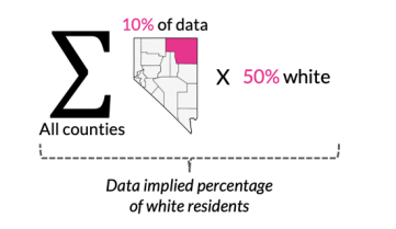
And the geography-wide percentage is the actual reported value for the percentage of white residents across all of Nevada. For the county-, state-, and national-level tools, these percentages are directly reported by the census (or calculated from census-reported counts for the appropriate numerator and denominator). This value is subtracted from the data-implied percentage to calculate the demographic disparity score.
Below is a pictorial representation for how the full demographic disparity score calculation is done for white residents in Nevada:

For just the city-level analysis, the geography-wide percentage is calculated from the tracts that compose the city, as our city boundary definitions may differ from the official Census boundaries.
Note
For analyses submitted via the API, the geography-wide percentage is calculated from the tracts that compose the geography for all geographic levels of analysis (city, county, state, and national). If a user submits variables from the American Community Survey as supplemental variables, they should note that the MOE calculated in this manner will differ from the MOE directly reported by the ACS for place-, county-, state-, and national-level estimates (see US Census Bureau 2020, 61).
Below is a mathematical and pictorial representation of the demographic disparity score as calculated for white residents in the city of Philadelphia. Note that the data-implied percentage is calculated the same way as for the county, state, and national tool, but the way the geography-wide percentage is calculated has changed.
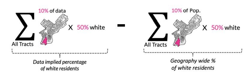
For the data-implied percentage, the share of white residents in each tract is an ACS variable with associated margin of error. Similarly, the geography-wide percentage uses the total geography population and the total white population in the geography, both of which are ACS variables with associated margins of error. To visualize this, you can rewrite the geography-wide percentage in the diagrams above as follows:
\[ geography-wide\ percentage\ (city)= \frac{\sum(number\ of\ white\ residents_i)}{\sum(total\ population_i)} \]
\[ geography-wide\ percentage\ (county,state,US) = \frac{number\ of\ white\ residents}{total\ population} \]
To take into account the variability in all these ACS figures, we calculate standard errors for the data-implied percentage and the geography-wide percentage using the relevant formulas from the ACS handbook. We then perform a test for statistical significance for the difference between these two ACS measures using a 95 percent confidence level.
We use the formula 3 from the ACS handbook (US Census Bureau 2020, chap. 7) to compute statistical significance, where X1 is the data-implied percentage, X2 is the geography-wide percentage, and ZCL is 1.96 (because we set a 95 percent confidence level).
\[If\ \Bigg| \frac{\hat{X_1} - {\hat{X_2}}}{\sqrt{[SE(\hat{X_1}) +SE(\hat{X_2})]^2}} \Bigg| >Z_{CL} \]
Next, we work through an example of the significance calculations for one of our demographic variables—the percentage of the total population that is white:
Imagine a geography with two census tracts, A and B. Census tract A contains 20 people, 15 of whom are white. Census tract B contains 25 people, 5 of whom are white. Also assume that tract A contains 30 percent of the data and tract B contains 70 percent of the data. The data-implied percentage for white residents would be \((0.3) * (15/20) + (0.7) * (5/25)\), or \(0.365\). If the selected geography were a city, the geography-wide percentage would be \((15 + 5) / (20 + 25)\), or \(0.444\). Note that for county, state, and national analysis, the numerator and denominator for the geography (or in some cases, the percentage itself of 0.444) would be directly reported. The demographic disparity score for white residents is \(0.365 − 0.444 = −0.079\).
Now assume that the margin of error for the percentage of white residents is 2 percent (0.02) in tract A is and 5 percent (0.05) in tract B. Using Equation 14.1 from the ACS handbook, and the fact that the data proportion is a constant number for each tract, the standard error for the data-implied percentage would be calculated as follows:
\[ SE(data\ implied\ percentage) = \frac{MOE(data\ implied\ percentage)}{1.645} = \frac{\sqrt{((0.3 * 0.02)^2 + (0.7 * 0.05)^2)}}{1.645} = 0.021 \]
We then need to calculate the standard error of the geography-wide percentage. For the county, state, and national analyses, the standard error may be directly reported (if the census directly reports the percentage estimate and associated margin of error) or can be calculated for the reported margins of error for the numerator (total white population) and denominator (total population) using Equation 14.2 as illustrated below. For the city-level analysis, we need to use the individual tract margins of error for the numerator and denominator to calculate the standard error of the geography-wide percentage as follows. Let’s assume that the margins of error for the population counts and white resident counts are as shown below:
Using Equation 14.1 from the ACS handbook for aggregating data across geographic areas, the MOE for the total city population would be \(\sqrt{5.52 + 52}\) , or \(7.43\), and the MOE for the total white resident population would be \(\sqrt{3.52 + 1.52}\) , or \(3.81\). Then using Equation 14.2, the standard error calculation for the geography-wide percentage of white residents would be
\[ SE(geography-wide\ percentage) = \frac{MOE(geography-wide\ percentage)}{1.645} = \frac{\sqrt{3.81^2 - \big(\frac{20^2}{45} * 7.43^2 \big)}} {45(1.645)} = 0.0255 \]
Now that we have the value and the standard errors for both the data-implied percentage and the geography-wide percentage, we perform a significance test with a 95 percent confidence level.
\[ Z_{CL} = \frac{0.444 - 0.365}{\sqrt{0.021^2 + 0.0255^2}} = 2.391 \]
This is larger than the critical value of 1.96, so we would report the demographic disparity of white residents at \(−0.079\) as statistically significant.